Goal
Create a chromosome-level synteny plot from orthologue assignments and genomic coordinates.
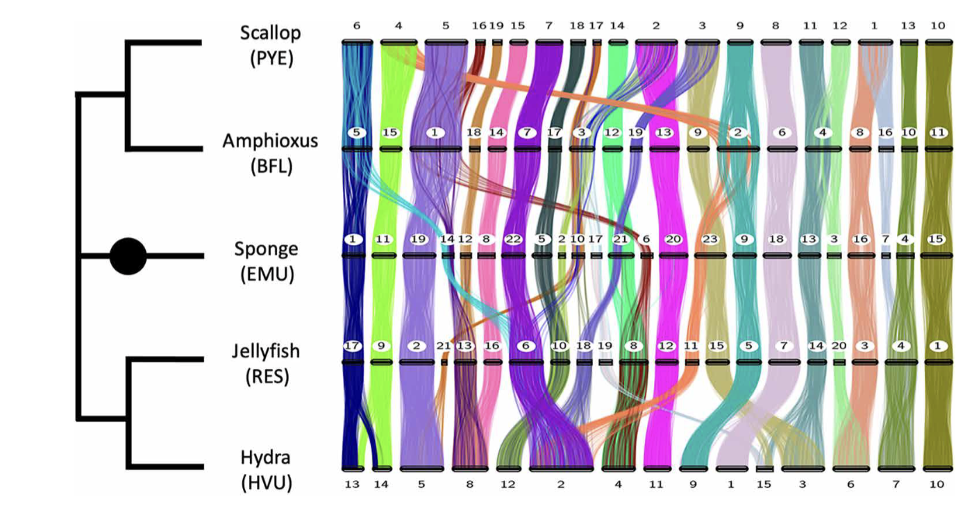
Workflow:
- Run extract_isoform pipelines for each species
- OrthoFinder
- Create coordinate files for each species
- Create karyotype files for each species
- Visualization using RIdeogram
Example:
OrthoFinder analysis
Run OrthoFinder on 4 species: Bfl, Ofu, Pma, Dja
Create a input directory and copy all four FASTA to the directory
mkdir orthofinder_input5

for species in Bfl Ofu Pma Dja; do
cp raw_data/processed_data/"${species}"_proteins_ReadyForOF.fa orthofinder_input5/"${species}"_proteins_ReadyForOF.fa
done
Run OrthoFinder
conda activate ///orthofinderorthofinder -f orthofinder_input5/ -t 100Results
1. Species tree
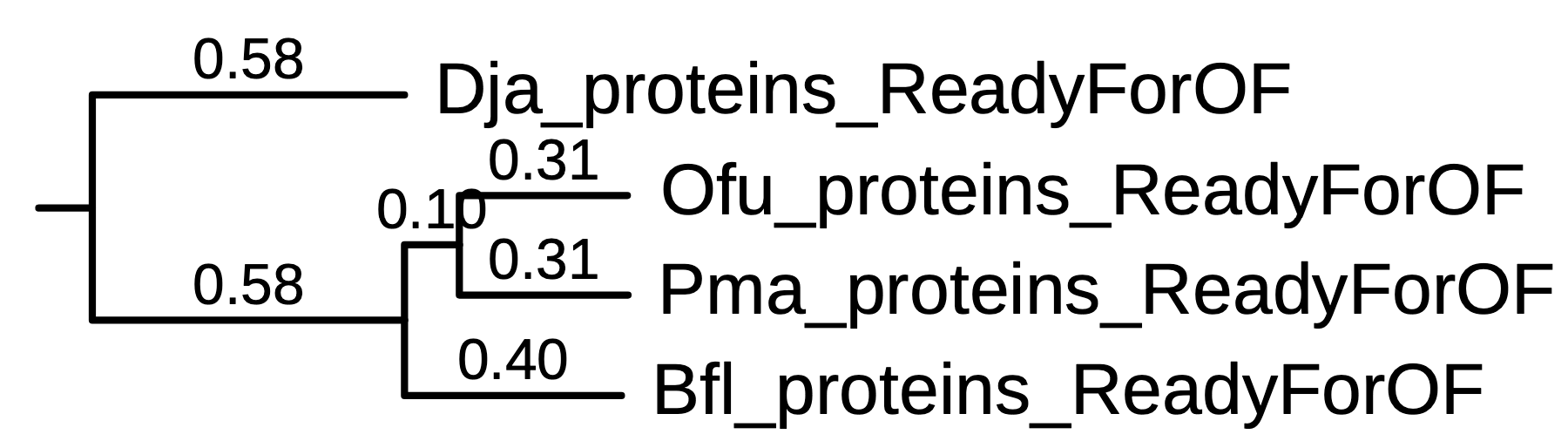
In TreeViewer, set Bfl as the outgroup, export the tree in Newick format, and place it back in the Species_Tree directory.
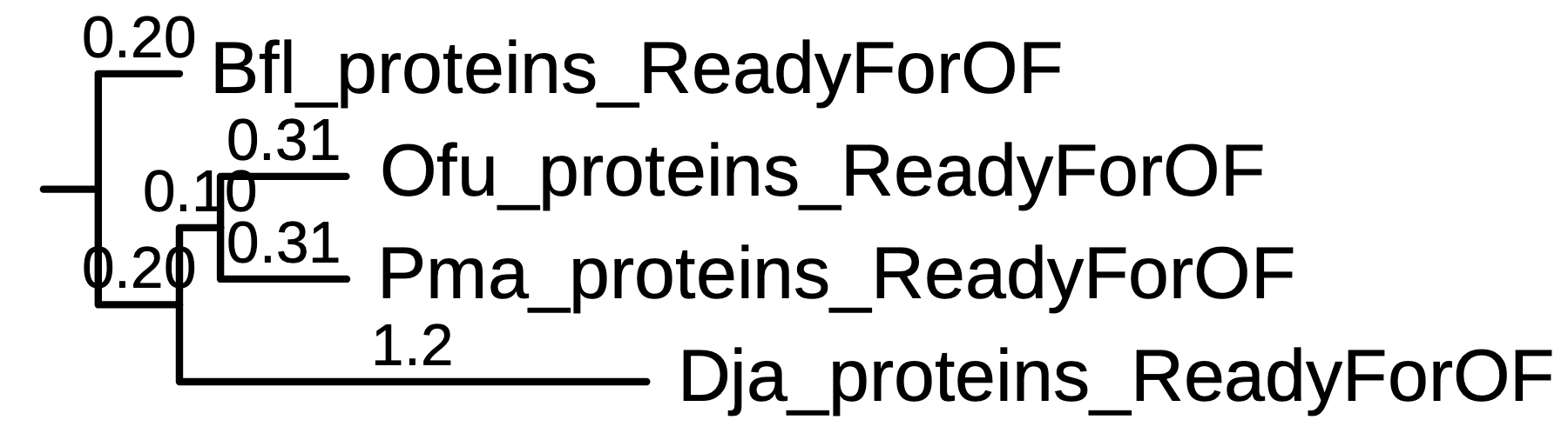
Rerun OrthoFinder using the revised tree.
orthofinder -ft orthofinder_input5/OrthoFinder/Results_Oct31/ -s orthofinder_input5/OrthoFinder/Results_Oct31/Species_Tree/SpeciesTree_rooted_new.nwk -t 100OrthoFinder creates Results_Oct31_1 containing the new N0.tsv result.
Earlier results:
2. Comparative_Genomics_Statistics/Statistics_Overall.tsv
In general it’s nice to see at least 80% of your genes assigned to orthogroups. Fewer than this means that you are probably missing orthology relationships that actually exist for some of the remaining genes, poor species sampling is the most likely cause for this.
Number of species       4
Number of genes 60095
Number of genes in orthogroups  48852
Number of unassigned genes      11243
Percentage of genes in orthogroups      81.3
Percentage of unassigned genes  18.7
Number of orthogroups   12821
Number of species-specific orthogroups  3416
Number of genes in species-specific orthogroups 18224
Percentage of genes in species-specific orthogroups     30.3
Mean orthogroup size    3.8
Median orthogroup size  3.0
G50 (assigned genes)    4
G50 (all genes) 3
O50 (assigned genes)    2938
O50 (all genes) 4576
Number of orthogroups with all species present  968
Number of single-copy orthogroups       655
3. Comparative_Genomics_Statistics/Statistics_PerSpecies.tsv
	    						Bfl_proteins_ReadyForOF Dja_proteins_ReadyForOF Ofu_proteins_ReadyForOF Pma_proteins_ReadyForOF
Number of genes 2361    4706    26876   26152
Number of genes in orthogroups  2357    3566    22196   20733
Number of unassigned genes      4       1140    4680    5419
Percentage of genes in orthogroups      99.8    75.8    82.6    79.3
Percentage of unassigned genes  0.2     24.2    17.4    20.7
Number of orthogroups containing species        2248    2747    11042   10873
Percentage of orthogroups containing species    17.5    21.4    86.1    84.8
Number of species-specific orthogroups  0       181     1735    1500
Number of genes in species-specific orthogroups 0       518     9727    7979
Percentage of genes in species-specific orthogroups 0.0 11.0 36.2 30.5- Species-specific orthogroup: An orthogroups that consist entirely of genes from one species = paralogs
New results after rerunning OrthoFinder (orthofinder_input5/OrthoFinder/Results_Oct31_1):
After rerunning:
1. Comparative_Genomics_Statistics/OrthologuesStats_one-to-one.tsv
number of one-to-one orthologues between each species pair.
                        Bfl_proteins_ReadyForOF Dja_proteins_ReadyForOF Ofu_proteins_ReadyForOF Pma_proteins_ReadyForOF
Bfl_proteins_ReadyForOF 0.0     829.0   2095.0  2061.0
Dja_proteins_ReadyForOF 829.0   0.0     1969.0  1884.0
Ofu_proteins_ReadyForOF 2095.0  1969.0  0.0     7963.0
Pma_proteins_ReadyForOF 2061.0  1884.0  7963.0  0.0
2. Phylogenetic_Hierarchical_Orthogroups/N0.tsv
orthofinder_input5/OrthoFinder/Results_Oct31/Orthogroups/Orthogroups_SingleCopyOrthologues.txt
The single-copy orthologue list appeared not to be regenerated after changing the tree, so this analysis reused the earlier list. The same files as the “Orthogroup Sequences” directory but restricted to only those orthogroups which contain exactly one gene per species.
OG0002110
OG0002111
OG0002113
OG0002114
OG0002115
OG0002117
OG0002119
OG0002122
OG0002123
OG0002124
Select the corresponding 654 rows from Results_Oct31_1/Phylogenetic_Hierarchical_Orthogroups/N0.tsv, the result produced with the revised tree.
Run
cat orthofinder_input5/OrthoFinder/Results_Oct31/Orthogroups/Orthogroups_SingleCopyOrthologues.txt | while read -r gene_id; do

orthologs=$(grep "\\b${gene_id}" orthofinder_input5/OrthoFinder/Results_Oct31_1/Phylogenetic_Hierarchical_Orthogroups/N0.tsv)

echo "$orthologs"

done > orthofinder_input5/OrthoFinder/Results_Oct31_1/Phylogenetic_Hierarchical_Orthogroups/N0_SCO.tsv
Example output:
N0.HOG0002215   OG0002110       n0      6520_J2_BL06899|Bfl     g2713|Dja       OFUS_LOCUS1605|Ofu      LOC117324952|Pma
N0.HOG0002216   OG0002111       n0      11339_J2_BL06923|Bfl    g2091|Dja       OFUS_LOCUS1167|Ofu      LOC117325306|Pma
N0.HOG0002218   OG0002113       n0      3366_J2_BL07026|Bfl     g574|Dja        OFUS_LOCUS2373|Ofu      LOC117325624|Pma
N0.HOG0002219   OG0002114       n0      11865_J2_BL07049|Bfl    g2473|Dja       OFUS_LOCUS2538|Ofu      LOC117324950|Pma
N0.HOG0002220   OG0002115       n0      6193_J2_BL07074|Bfl     g3957|Dja       OFUS_LOCUS2360|Ofu      LOC117325966|Pma
N0.HOG0002222   OG0002117       n0      3933_C1_BL07115|Bfl     g1453|Dja       OFUS_LOCUS20833|Ofu     LOC117335045|Pma
N0.HOG0002224   OG0002119       n0      12777_C1_BL07176|Bfl    g3843|Dja       OFUS_LOCUS21278|Ofu     LOC117334956|Pma
N0.HOG0002227   OG0002122       n0      6832_C1_BL07212|Bfl     g3940|Dja       OFUS_LOCUS21796|Ofu     LOC117335235|Pma
N0.HOG0002228   OG0002123       n0      9374_C1_BL07224|Bfl     g532|Dja        OFUS_LOCUS21306|Ofu     LOC117334621|Pma
Keep only columns 2 and 4–7 for the next step.
mkdir RIdeogram5
awk '{print $2, $4, $5, $6, $7}' orthofinder_input5/OrthoFinder/Results_Oct31_1/Phylogenetic_Hierarchical_Orthogroups/N0_SCO.tsv > RIdeogram5/N0_SCO.tsv
OG0002110 6520_J2_BL06899|Bfl g2713|Dja OFUS_LOCUS1605|Ofu LOC117324952|Pma
OG0002111 11339_J2_BL06923|Bfl g2091|Dja OFUS_LOCUS1167|Ofu LOC117325306|Pma
OG0002113 3366_J2_BL07026|Bfl g574|Dja OFUS_LOCUS2373|Ofu LOC117325624|Pma
OG0002114 11865_J2_BL07049|Bfl g2473|Dja OFUS_LOCUS2538|Ofu LOC117324950|Pma
OG0002115 6193_J2_BL07074|Bfl g3957|Dja OFUS_LOCUS2360|Ofu LOC117325966|Pma
OG0002117 3933_C1_BL07115|Bfl g1453|Dja OFUS_LOCUS20833|Ofu LOC117335045|Pma
OG0002119 12777_C1_BL07176|Bfl g3843|Dja OFUS_LOCUS21278|Ofu LOC117334956|Pma
OG0002122 6832_C1_BL07212|Bfl g3940|Dja OFUS_LOCUS21796|Ofu LOC117335235|Pma
OG0002123 9374_C1_BL07224|Bfl g532|Dja OFUS_LOCUS21306|Ofu LOC117334621|Pma
OG0002124 11085_C1_BL07258|Bfl g265|Dja OFUS_LOCUS20751|Ofu LOC117335236|PmaCoordinate files for each species
Process the SCO file from the output of OrthoFinder
RIdeogram5/N0_SCO.tsv
OG0002110 6520_J2_BL06899|Bfl g2713|Dja OFUS_LOCUS1605|Ofu LOC117324952|Pma
OG0002111 11339_J2_BL06923|Bfl g2091|Dja OFUS_LOCUS1167|Ofu LOC117325306|Pma
OG0002113 3366_J2_BL07026|Bfl g574|Dja OFUS_LOCUS2373|Ofu LOC117325624|Pma
OG0002114 11865_J2_BL07049|Bfl g2473|Dja OFUS_LOCUS2538|Ofu LOC117324950|Pma
OG0002115 6193_J2_BL07074|Bfl g3957|Dja OFUS_LOCUS2360|Ofu LOC117325966|Pma
OG0002117 3933_C1_BL07115|Bfl g1453|Dja OFUS_LOCUS20833|Ofu LOC117335045|Pma
OG0002119 12777_C1_BL07176|Bfl g3843|Dja OFUS_LOCUS21278|Ofu LOC117334956|Pma
OG0002122 6832_C1_BL07212|Bfl g3940|Dja OFUS_LOCUS21796|Ofu LOC117335235|Pma
OG0002123 9374_C1_BL07224|Bfl g532|Dja OFUS_LOCUS21306|Ofu LOC117334621|Pma
OG0002124 11085_C1_BL07258|Bfl g265|Dja OFUS_LOCUS20751|Ofu LOC117335236|Pma- Omit orthology ID
- Split the Bfl ID (
10079_C1_BL07110|Bfl) cased 0n “_” - Split it to 4 species** (with ALG ID)**
awk '{print $2, $3, $4, $5}' RIdeogram5/N0_SCO.tsv | awk '{ split($1,a,"_"); print a[1], a[2],a[3]} ' > RIdeogram5/N0_SCO_Bfl.tsv
awk '{print $2, $3, $4, $5}' RIdeogram5/N0_SCO.tsv | awk '{ split($1,a,"_"); print a[1], a[2], $2} ' > RIdeogram5/N0_SCO_Dja.tsv
awk '{print $2, $3, $4, $5}' RIdeogram5/N0_SCO.tsv | awk '{ split($1,a,"_"); print a[1], a[2], $3} ' > RIdeogram5/N0_SCO_Ofu.tsv
awk '{print $2, $3, $4, $5}' RIdeogram5/N0_SCO.tsv | awk '{ split($1,a,"_"); print a[1], a[2], $4} ' > RIdeogram5/N0_SCO_Pma.tsv
Process Amphioxus (Bfl)
Remove the |Bfl suffix.
sed -i 's/|Bfl//' RIdeogram5/N0_SCO_Bfl.tsvSelect annotation rows whose third column is gene.
Split column 9 at semicolons and retain the attribute beginning with gene_id.
awk -F "\t" '$3 == "gene"' raw_data/Braflo_7u5tJ.gtf | awk -F "\t" '{split($9,a,";"); gene=""; for (i in a) {if (a[i] ~ /^gene_id/){ gene=a[i]}} print $1,$4,$5,gene }' > RIdeogram5/Bfl_processed_GTF.txtMatch the single-copy orthologue list against RIdeogram5/Bfl_processed_GTF.txt.
awk 'NR==FNR {a[$3]=$1"\t"$2; next;} {gsub(/"/, "", $5); if ($5 in a) {print $1, $2, $3, $5, a[$5]}}' RIdeogram5/N0_SCO_Bfl.tsv RIdeogram5/Bfl_processed_GTF.txt | awk -F " " '{print $5, "Complete", $1, $2, $3, $6}' OFS="\t" > RIdeogram5/Bfl_Coor_ReadyForRIdeo.txtExample output
12048   Complete        Sc7u5tJ_1336    162669  209110  O2
10566   Complete        Sc7u5tJ_1398    7212731 7231532 B3
12811   Complete        Sc7u5tJ_1398    8651415 8669381 B3
6694    Complete        Sc7u5tJ_1398    11358893        11386485        B3
4273    Complete        Sc7u5tJ_1398    14579113        14595426        B3
1880    Complete        Sc7u5tJ_1398    14740932        14754077        B3
4146    Complete        Sc7u5tJ_1398    14806693        14814071        B3
**Process Pma **
Remove the |Pma suffix.
sed -i 's/|Pma//' RIdeogram5/N0_SCO_Pma.tsv6520 J2 LOC117324952
11339 J2 LOC117325306
3366 J2 LOC117325624
11865 J2 LOC117324950
6193 J2 LOC117325966
3933 C1 LOC117335045
12777 C1 LOC117334956
6832 C1 LOC117335235
9374 C1 LOC117334621Select annotation rows whose third column is gene.
Split column 9 at semicolons and extract the gene identifier. The command below uses Name=.
awk -F "\t" '$3 == "gene"' raw_data/Pma.gff | awk -F "\t" '{split($9,a,";"); gene=""; for (i in a) {if (a[i] ~ /^Name=/){ gene=a[i]}} print $1,$4,$5,gene }' > RIdeogram5/Pma_processed_GTF.txtMatch the processed annotation against the single-copy orthologue list.
awk 'NR==FNR {a[$3]=$1"\t"$2; next;} {gsub(/Name=/, "", $4); if ($4 in a) print $1, $2, $3, $4, a[$4]}' RIdeogram5/N0_SCO_Pma.tsv RIdeogram5/Pma_processed_GTF.txt | awk -F " " '{print $5, "Complete", $1, $2, $3, $6}' OFS="\t" > RIdeogram5/Pma_Coor_ReadyForRIdeo.txtExample output
4440    Complete        NC_047015.1     6783625 6794099 H
888     Complete        NC_047015.1     8214924 8217938 H
11379   Complete        NC_047015.1     9297388 9319037 H
9901    Complete        NC_047015.1     9342300 9362632 H
5495    Complete        NC_047015.1     9530591 9555679 H
6695    Complete        NC_047015.1     11742530        11748020        Qa
1187    Complete        NC_047015.1     11771800        11774492        Qd
Process Ofu
Remove the |Ofu suffix.
sed -i 's/|Ofu//' RIdeogram5/N0_SCO_Ofu.tsv6520 J2 OFUS_LOCUS1605
11339 J2 OFUS_LOCUS1167
3366 J2 OFUS_LOCUS2373
11865 J2 OFUS_LOCUS2538
6193 J2 OFUS_LOCUS2360
3933 C1 OFUS_LOCUS20833
12777 C1 OFUS_LOCUS21278Select annotation rows whose third column is gene.
Split column 9 at semicolons and extract the gene identifier. The command below uses Name=.
awk -F "\t" '$3 == "gene"' raw_data/Ofu.gff | awk -F "\t" '{split($9,a,";"); gene=""; for (i in a) {if (a[i] ~ /^Name=/){ gene=a[i]}} print $1,$4,$5,gene }' > RIdeogram5/Ofu_processed_GTF.txtExample output:
CAIIXF020000001.1 1176 110407 Name=OFUS_LOCUS1
CAIIXF020000001.1 116850 181090 Name=OFUS_LOCUS2
CAIIXF020000001.1 181092 204819 Name=OFUS_LOCUS3
CAIIXF020000001.1 210128 363898 Name=OFUS_LOCUS4
CAIIXF020000001.1 287204 289991 Name=OFUS_LOCUS5
CAIIXF020000001.1 342283 344093 Name=OFUS_LOCUS6
CAIIXF020000001.1 370001 371202 Name=OFUS_LOCUS7
CAIIXF020000001.1 381000 436743 Name=OFUS_LOCUS8
Match the processed annotation against the single-copy orthologue list.
awk 'NR==FNR {a[$3]=$1"\t"$2; next;} {gsub(/Name=/, "", $4); if ($4 in a) print $1, $2, $3, $4, a[$4]}' RIdeogram5/N0_SCO_Ofu.tsv RIdeogram5/Ofu_processed_GTF.txt | awk -F " " '{print $5, "Complete", $1, $2, $3, $6}' OFS="\t" > RIdeogram5/Ofu_Coor_ReadyForRIdeo.txtExample output
7788    Complete        CAIIXF020000001.1       1498871 1517991 P
5980    Complete        CAIIXF020000001.1       2260062 2287167 J1
10751   Complete        CAIIXF020000001.1       3325189 3362254 J1
4222    Complete        CAIIXF020000001.1       3801787 3811693 L
8931    Complete        CAIIXF020000001.1       4403016 4408822 L
Process Dja
Remove the |Dja suffix.
sed -i 's/|Dja//' RIdeogram5/N0_SCO_Dja.tsvSelect annotation rows whose third column is gene.
Split column 9 at semicolons and retain the attribute beginning with ID=.
awk -F "\t" '$3 == "gene"' raw_data/Dja.gff | awk -F "\t" '{split($9,a,";"); gene=""; for (i in a) {if (a[i] ~ /^ID=/){ gene=a[i]}} print $1,$4,$5,gene }' > RIdeogram5/Dja_processed_GTF.txtExample output:
SCAFFOLD1 69875 71212 ID=g1
SCAFFOLD1 72736 114086 ID=g2
SCAFFOLD1 197096 197824 ID=g3
SCAFFOLD1 209906 211248 ID=g4
SCAFFOLD1 212293 213652 ID=g5
SCAFFOLD1 212293 213652 ID=g6
SCAFFOLD1 228716 233096 ID=g7
SCAFFOLD1 233176 233979 ID=g8
SCAFFOLD1 245667 246412 ID=g9
SCAFFOLD1 251026 253622 ID=g10
Match the processed annotation against the single-copy orthologue list.
awk 'NR==FNR {a[$3]=$1"\t"$2; next;} {gsub(/ID=/, "", $4); if ($4 in a) print $1, $2, $3, $4, a[$4]}' RIdeogram5/N0_SCO_Dja.tsv RIdeogram5/Dja_processed_GTF.txt | awk -F " " '{print $5, "Complete", $1, $2, $3, $6}' OFS="\t" > RIdeogram5/Dja_Coor_ReadyForRIdeo.txtExample output
3645    Complete        SCAFFOLD1       72736   114086  Eb
1538    Complete        SCAFFOLD1       209906  211248  Qa
2244    Complete        SCAFFOLD1       518199  519050  H
9979    Complete        SCAFFOLD1       620799  622273  Ea
11400   Complete        SCAFFOLD1       633069  634411  C1
5689    Complete        SCAFFOLD1       686978  688985  A2
789     Complete        SCAFFOLD1       905722  910826  M
Karyotype files for each species
Goal:
To create karyotype files for 4 speceis like this:
Chr	Start	End	species	size	color
chr1	1	71920973	lan	12	25252
chr2	1	49367315	lan	12	25252
chr3	1	34252355	lan	12	25252
chr4	1	30086056	lan	12	25252
chr5	1	25664212	lan	12	25252
.
.
(although in Vignettes of RIdeogram it presents the file like this)
Chr Start       End  CE_start    CE_end
1     0 248956422 122026459 124932724
2     0 242193529  92188145  94090557
3     0 198295559  90772458  93655574
4     0 190214555  49712061  51743951
5     0 181538259  46485900  50059807
6     0 170805979  58553888  59829934
Example - Bfl:
Create a chromosome list
awk -F "\t" ' $3 == "gene" ' raw_data/Braflo_7u5tJ.gtf | awk -F "\t" '{print $1}' | sort -k1,1 -u > raw_data/Bfl_chr_list.txtSc7u5tJ_1007
Sc7u5tJ_1014
Sc7u5tJ_1022
Sc7u5tJ_1025
Sc7u5tJ_1033
Sc7u5tJ_1041
Sc7u5tJ_1044
.
.Get the start and end for each chromosome ID
cat raw_data/Bfl_chr_list.txt | while read -r chr_ID; do

chr_start_end=$(grep "${chr_ID}\\b" <(awk -F "\t" ' $3 == "gene" ' raw_data/Braflo_7u5tJ.gtf) | sort -k4,4n -k5,5n | awk ' {if (FNR == 1) {start = $4; end = $5; chr = $1} else { end = $5}}  END {print chr, start, end}' OFS="\t" )

echo "$chr_start_end"

done > RIdeogram/Bfl_Karyotype.txt- Read each chromosome ID from
raw_data/Bfl_chr_list.txt. - Search the gene-only GTF rows for that ID and extract the chromosome identifier and the recorded start and end positions.
- Use a word boundary in the chromosome-ID match, so that
Sc7u5tJ_102does not also matchSc7u5tJ_1022. - Sort the matching genes by start position, then end position. The command records the first row’s start and the final row’s end.
The
awkexpression in the command performs the following steps: On the first row (FNR == 1), record the chromosome ID, start, and end. For each later row, overwrite the stored end with column 5. The final output therefore uses the last row’s end. This assumes that end is the largest observed end; nested or overlapping genes would require an explicit maximum instead. For example, the genes onSc7u5tJ_97are:
- Use a word boundary in the chromosome-ID match, so that
Sc7u5tJ_97      EVM     gene    5723    7962    .       -       .       gene_id "BL22973"; copy_id "BL22973_1"; coverage "1.0"; sequence_ID "1.0"; extra_copy_number "0";
Sc7u5tJ_97      EVM     gene    9101    10795   .       -       .       gene_id "BL22972"; copy_id "BL22972_1"; coverage "1.0"; sequence_ID "1.0"; extra_copy_number "0";
Sc7u5tJ_97      EVM     gene    11209   12522   .       -       .       gene_id "BL22971"; copy_id "BL22971_1"; coverage "1.0"; sequence_ID "1.0"; extra_copy_number "0";
Sc7u5tJ_97      EVM     gene    18441   41685   .       +       .       gene_id "BL22970"; copy_id "BL22970_1"; coverage "1.0"; sequence_ID "1.0"; extra_copy_number "0";
Example output:
Sc7u5tJ_97 5723 41685Find the longest chromosomes
Add a column containing end − start, then sort by this recorded span.
awk '{ print $0, $3-$2} ' RIdeogram/Bfl_Karyotype.txt OFS="\t" | sort -k4,4n | tail -25Sc7u5tJ_1560 3436 653616 650180
Sc7u5tJ_1585 10324 689725 679401
Sc7u5tJ_1578 2838 720191 717353
Sc7u5tJ_1495 13255 813858 800603
Sc7u5tJ_1421 2628 913497 910869
Sc7u5tJ_1439 1116 1648760 1647644
Sc7u5tJ_417 147 17113240 17113093
Sc7u5tJ_1398 1561 18548748 18547187
Sc7u5tJ_190 1954 19085550 19083596
Sc7u5tJ_1485 4732 19116635 19111903
Sc7u5tJ_1579 39018 21508007 21468989
Sc7u5tJ_1442 3025 21809174 21806149
Sc7u5tJ_1552 50612 22406760 22356148
Sc7u5tJ_566 2719 22971665 22968946
Sc7u5tJ_1565 2261 23528568 23526307
Sc7u5tJ_350 814 23930091 23929277
Sc7u5tJ_1517 17218 25441410 25424192
Sc7u5tJ_320 2980 25570490 25567510
Sc7u5tJ_1559 21678 25952566 25930888
Sc7u5tJ_1571 18280 28085416 28067136
Sc7u5tJ_1587 5980 29544808 29538828
Sc7u5tJ_366 6705 34237864 34231159
Sc7u5tJ_1568 169 34244043 34243874
Sc7u5tJ_1590 9817 35134533 35124716
Sc7u5tJ_339 2514 35329414 35326900The span drops sharply between Sc7u5tJ_417 and Sc7u5tJ_1439: 17,113,093 to 1,647,644.
The analysis therefore selected 19 chromosomes for this visualization.
Keep the chromosome ID and size, then add the required columns and column names
awk '{ print $0, $3-$2} ' RIdeogram/Bfl_Karyotype.txt OFS="\t" | sort -k4,4n | tail -19 | awk 'BEGIN {OFS="\t"; print "Chr", "Start", "End", "species", "size", "color"} {print $1, 1, $4, "bfl", 12, 25252}' OFS="\t" > RIdeogram/Bfl_Karyotype_ReadyForRIdeo.txtChr Start End species size color
Sc7u5tJ_417 1 17113093 bfl 12 25252
Sc7u5tJ_1398 1 18547187 bfl 12 25252
Sc7u5tJ_190 1 19083596 bfl 12 25252
Sc7u5tJ_1485 1 19111903 bfl 12 25252
Sc7u5tJ_1579 1 21468989 bfl 12 25252
Sc7u5tJ_1442 1 21806149 bfl 12 25252
Sc7u5tJ_1552 1 22356148 bfl 12 25252
Sc7u5tJ_566 1 22968946 bfl 12 25252
Sc7u5tJ_1565 1 23526307 bfl 12 25252
Sc7u5tJ_350 1 23929277 bfl 12 25252
Sc7u5tJ_1517 1 25424192 bfl 12 25252
Sc7u5tJ_320 1 25567510 bfl 12 25252
Sc7u5tJ_1559 1 25930888 bfl 12 25252
Sc7u5tJ_1571 1 28067136 bfl 12 25252
Sc7u5tJ_1587 1 29538828 bfl 12 25252
Sc7u5tJ_366 1 34231159 bfl 12 25252
Sc7u5tJ_1568 1 34243874 bfl 12 25252
Sc7u5tJ_1590 1 35124716 bfl 12 25252
Sc7u5tJ_339 1 35326900 bfl 12 25252Visualization with RIdeogram
Collect all input files for RIdeogram in one directory.
Example (Bfl vs Hvu)
RIdeogram script from Isabel
# Assign source and target species
source <- "Bfl"
target <- "Hvu"

# If you would like to reorder the chromosomes, put the chromosome order here.
# Otherwise, set reorder to FALSE
reorder <- FALSE
#bfl_order <- c(4,11,2,15,19,9,3,13,18,1,16,8,7,6,10,5,17,14,12)
#pma_order <- c(10,12,8,9,4,5,17,1,19,3,13,2,6,11,15,7,18,16,14)
#llo_order <- c(8,6,2,4,5,14,1,17,3,18,13,16,9,11,15,7,19,12,10)
#lan_order <- c(1,2,7,3,4,5,6,8,9,10)
#source_order <- lan_order
#target_order <- pma_order
Set karyotypes
# Load karyotype files
source_karyotype <- read.table(paste0("RIdeogram/input/", source, "_Karyotype_ReadyForRIdeo.txt"),
                              sep = "\t", header = TRUE, stringsAsFactors = F)
target_karyotype <- read.table(paste0("RIdeogram/input/", target, "_Karyotype_ReadyForRIdeo.txt"),
                              sep = "\t", header = TRUE, stringsAsFactors = F)

# Sort karyotypes such that chromosomes are ordered from largest to smallest
source_karyotype <- source_karyotype[order(source_karyotype$End,
                                           decreasing = TRUE), ]
target_karyotype <- target_karyotype[order(target_karyotype$End,
                                           decreasing = TRUE), ]

# Create dictionaries such that each karyotype name can be mapped to an integer
source_mapping <- setNames(1:nrow(source_karyotype), source_karyotype$Chr)
target_mapping <- setNames(1:nrow(target_karyotype), target_karyotype$Chr)

# Save the original chromosome names to a new column
source_karyotype$orig_ids <- source_karyotype$Chr
target_karyotype$orig_ids <- target_karyotype$Chr

# Remap the karyotypes such that the names are integers
source_karyotype$Chr <- source_mapping[source_karyotype$Chr]
target_karyotype$Chr <- target_mapping[target_karyotype$Chr]

# Reorder karyotypes as specified.
# Create a mapping to link karyotype to order of appearance
if (reorder == TRUE) {
    source_karyotype <- source_karyotype[order(match(source_karyotype$Chr, source_order)),]
    target_karyotype <- target_karyotype[order(match(target_karyotype$Chr, target_order)),]

    source_remap <- setNames(1:nrow(source_karyotype), source_order)
    target_remap <- setNames(1:nrow(target_karyotype), target_order)
}

# Combine the karyotypes into one matrix
karyotype_all <- rbind(source_karyotype, target_karyotype,
                        make.row.names=FALSE)
karyotype_all$orig_ids <- NULL
# Set fill colours for nodes
karyotype_all$fill <- "cccccc"

# Reorder the columns
karyotype_all <- karyotype_all[, c(1,2,3,7,4,5,6)]

# Change the datatype of of the variables into a data frame
karyotype_all <- as.data.frame(karyotype_all, stringsAsFactors = F )
karyotype_all
Set genes
# Load coordinates files
source_coords <- read.table(paste0("RIdeogram/input/", source, "_Coor_ReadyForRIdeo.txt"),
                            sep = "\\t", header = FALSE, stringsAsFactors = F)
target_coords <- read.table(paste0("RIdeogram/input/", target, "_Coor_ReadyForRIdeo.txt"),
                            sep = "\\t", header = FALSE, stringsAsFactors = F)

# Check file length
nrow(source_coords)
nrow(target_coords)

# Get rid of coordinates that aren't on the selected chromosomes
# this might chanege
source_coords <- source_coords[source_coords$V3 %in% source_karyotype$orig_ids,]
target_coords <- target_coords[target_coords$V3 %in% target_karyotype$orig_ids,]

# Recheck file length
nrow(source_coords)
nrow(target_coords)


# Map the chromosome names to appropriate karyotype numbers for both coordinate sets
source_coords$V3 <- source_mapping[source_coords$V3]
target_coords$V3 <- target_mapping[target_coords$V3]

# Remap the chromosomes to the reshuffled chromosome order if necessary
if (reorder == TRUE) {
    source_coords$V3 <- source_remap[as.character(source_coords$V3)]
    target_coords$V3 <- target_remap[as.character(target_coords$V3)]
}


# Check coordinates file
source_coords
target_coords
# Create connections
coords_all <- merge(source_coords, target_coords, by = "V1")[, c(-1, -2, -6,-7)] # SOURCE 一定要放前面
# Relabel columns
colnames(coords_all) <- c( "Species_1", "Start_1", "End_1", "Species_2", "Start_2", "End_2","ALG")
# species 1 就是 source
coords_allCreate ALG colour map
alg_hexmap <- c("A1a" = "A6CDE3", "A1b" = "A6CDE3", "A2" = "197AB4",
                "B1" = "089E78", "B2" = "31A149", "B3" = "B2D287",
                "C1" = "F19799", "C2" = "E42027",
                "D"  = "F7F09B",
                "Ea" = "AF5B2A", "Eb" = "AF5B2A",
                "F"  = "DA6227",
                "G"  = "7671B0",
                "H"  = "E42C8A",
                "I"  = "65A744",
                "J1" = "C9B2D3", "J2" = "664292",
                "K"  = "E6AB22",
                "L"  = "A4782B",
                "M"  = "90CDC3",
                "N"  = "686868",
                "O1" = "EF7E25", "O2" = "F9BD6F",
                "P"  = "BDB9DA",
                "Qa" = "FED832", "Qb" = "FED832", "Qc" = "FED832", "Qd" = "FED832",
                "R"  = "00008B")

# Reassign line colours based on the mapping above
coords_all$fill <- alg_hexmap[coords_all$ALG]
Filter out the jumping genes to reduce noise
coords_all <- coords_all %>%
    group_by(Species_1, Species_2) %>%
    filter(n() > 5) %>%
    ungroup()

coords_all_output <- coords_all

colnames(coords_all_output) = c(source, "start_1", "End_1", target, "Start_2", "End_2", "ALG", "ALG_ColorCode")

write_csv(coords_all_output, file = paste0(output_dir,  source , "_", target , "_synteny_table.csv"))
Prepare to plot
# Re-order connections by colour
coords_all <- coords_all[with(coords_all, order(fill)),]

# Remove the 7th column and reformat into data frame to plot
synteny_coord <- as.data.frame(coords_all[,-7])
Plot
# Create synteny plot
ideogram(karyotype = karyotype_all,
         synteny = synteny_coord,
         output = paste0("RIdeogram/output/", source, "_", target, "_synteny.svg"))
?ideogram()
# Convert svg file to pdf
convertSVG(paste0("RIdeogram/output/", source, "_", target, "_synteny.svg"),
           file = paste0("RIdeogram/output/", source, "_", target, "_synteny.pdf"),
           device = "pdf")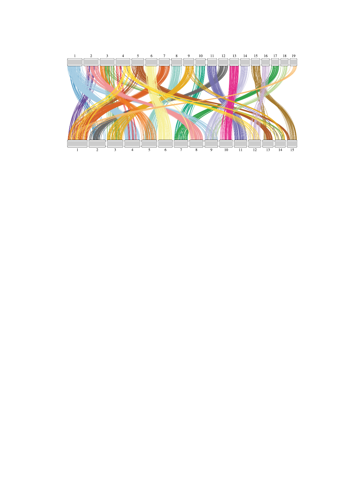
Bfl is shown at the top and Hvu at the bottom.