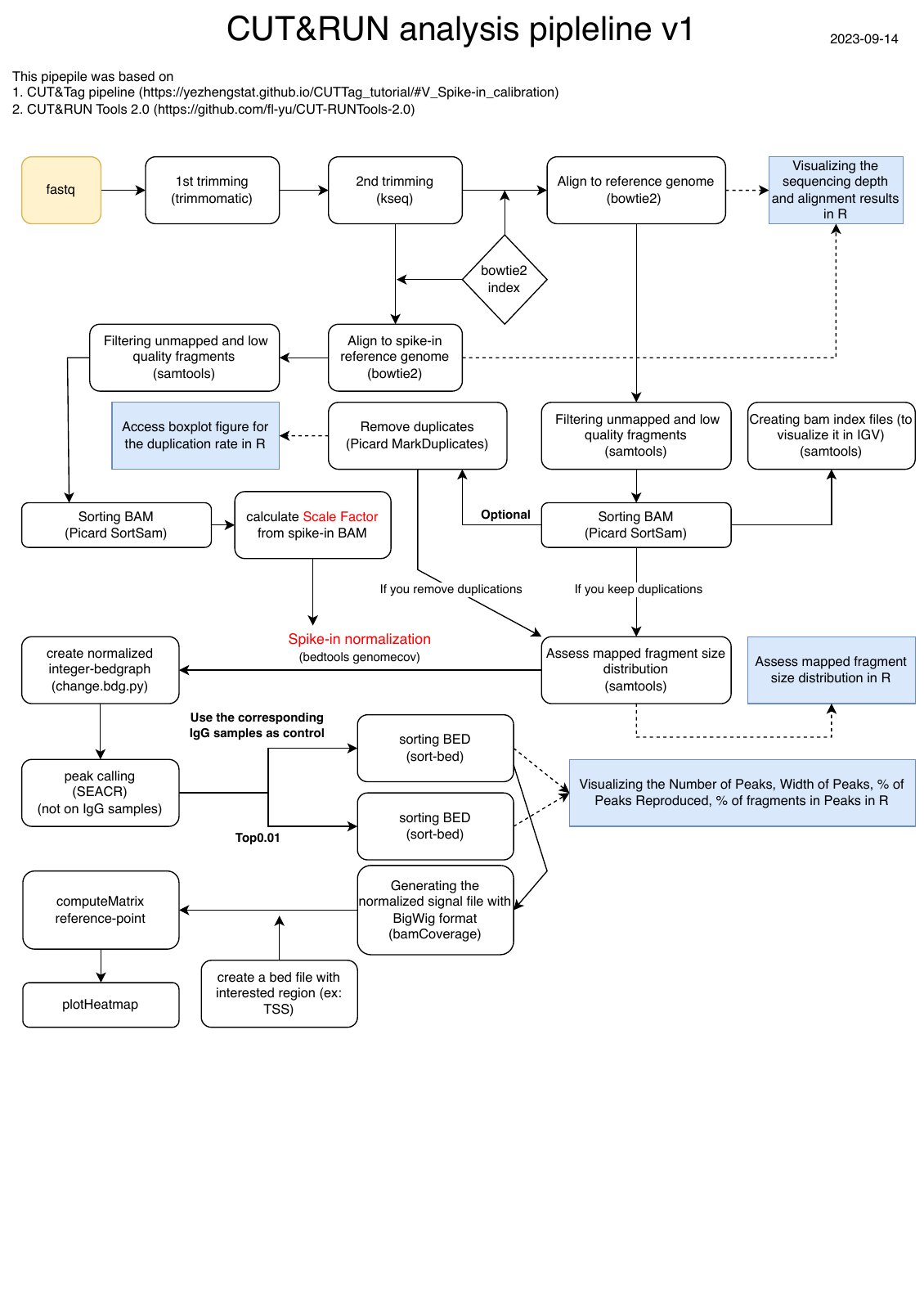
Workflow
Sample
The recorded sample panel contains five antibody labels, each in wild-type (WT) and conditional-knockout (cko) samples. The table retains those labels, including the Rbp1 spelling used in the sample list.
| Target | Treatment |
|---|---|
| Epcam | WT |
| Epcam | cko |
| H3K4me3 | WT |
| H3K4me3 | cko |
| IgG | WT |
| IgG | cko |
| Non_p | WT |
| Non_p | cko |
| Rbp1 | WT |
| Rbp1 | cko |
- Epcam (Epithelial Cell Adhesion Molecule): the experiment labels one antibody group Epcam. Epcam is a cell-surface protein; the interpretation of this label in a chromatin-profiling assay requires the experimental antibody and target information. It should not, by itself, be read as evidence of direct Epcam DNA binding.
- H3K4me3 (Tri-methylation of lysine 4 on histone H3): This is a specific histone modification associated with actively transcribed genes. Histone modifications are critical for regulating DNA accessibility and gene expression. By analyzing H3K4me3, you’re likely investigating the locations of active transcription and how this changes between wild type and knockout conditions.
- Non-p: the label is retained from the experiment. The notes suggest a non-phosphorylated target, but the exact protein or epitope is not specified.
- IgG (Immunoglobulin G): IgG is used as a negative control in CUT&RUN assays. Since IgG is a general antibody that should not specifically bind to any particular protein of interest in your sample, any DNA fragments pulled down in this condition are considered background noise. This helps to discern specific interactions from nonspecific background signals.
- Rpb1 (RNA polymerase II subunit B1): Rpb1 is a component of RNA polymerase II, the enzyme responsible for transcribing most eukaryotic genes into mRNA. Targeting Rpb1 in CUT&RUN can reveal the binding sites of the polymerase across the genome, highlighting regions of active transcription or regulatory elements being influenced by the presence or absence of certain genes. (SEACR is intended to call peaks and enriched regions from sparse CUT&RUN or chromatin profiling data in which background is dominated by “zeroes” (i.e. regions with no read coverage)
Use all the samples Epcam/H3K4me3/Non-p/IgG/Rpb1
Second stage trimming (optional)
-
kseq (
fastq_sequence_length: 50**)**trimming1Path="###" ~/Shared/CUTandRUN_Wu_Kao_20230828/CUT-RUNTools-2.0-master/install/kseq_test $trimming1Path/PH04_trimmed_R1_paired.fq 50 results/trimming2/Epcam_WT1_1.paired.fastq.gz && ~/Shared/CUTandRUN_Wu_Kao_20230828/CUT-RUNTools-2.0-master/install/kseq_test $trimming1Path/PH04_trimmed_R2_paired.fq 50 results/trimming2/Epcam_WT1_2.paired.fastq.gz && ~/Shared/CUTandRUN_Wu_Kao_20230828/CUT-RUNTools-2.0-master/install/kseq_test $trimming1Path/PH09_trimmed_R1_paired.fq 50 results/trimming2/Epcam_WT2_1.paired.fastq.gz && ~/Shared/CUTandRUN_Wu_Kao_20230828/CUT-RUNTools-2.0-master/install/kseq_test $trimming1Path/PH09_trimmed_R2_paired.fq 50 results/trimming2/Epcam_WT2_2.paired.fastq.gz && ~/Shared/CUTandRUN_Wu_Kao_20230828/CUT-RUNTools-2.0-master/install/kseq_test $trimming1Path/PW04_trimmed_R1_paired.fq 50 results/trimming2/Epcam_cko1_1.paired.fastq.gz && ~/Shared/CUTandRUN_Wu_Kao_20230828/CUT-RUNTools-2.0-master/install/kseq_test $trimming1Path/PW04_trimmed_R2_paired.fq 50 results/trimming2/Epcam_cko1_2.paired.fastq.gz && ~/Shared/CUTandRUN_Wu_Kao_20230828/CUT-RUNTools-2.0-master/install/kseq_test $trimming1Path/PW09_trimmed_R1_paired.fq 50 results/trimming2/Epcam_cko2_1.paired.fastq.gz && ~/Shared/CUTandRUN_Wu_Kao_20230828/CUT-RUNTools-2.0-master/install/kseq_test $trimming1Path/PW09_trimmed_R2_paired.fq 50 results/trimming2/Epcam_cko2_2.paired.fastq.gz && ~/Shared/CUTandRUN_Wu_Kao_20230828/CUT-RUNTools-2.0-master/install/kseq_test $trimming1Path/PH02_trimmed_R1_paired.fq 50 results/trimming2/H3K4me3_WT1_1.paired.fastq.gz && ~/Shared/CUTandRUN_Wu_Kao_20230828/CUT-RUNTools-2.0-master/install/kseq_test $trimming1Path/PH02_trimmed_R2_paired.fq 50 results/trimming2/H3K4me3_WT1_2.paired.fastq.gz && ~/Shared/CUTandRUN_Wu_Kao_20230828/CUT-RUNTools-2.0-master/install/kseq_test $trimming1Path/PH07_trimmed_R1_paired.fq 50 results/trimming2/H3K4me3_WT2_1.paired.fastq.gz && ~/Shared/CUTandRUN_Wu_Kao_20230828/CUT-RUNTools-2.0-master/install/kseq_test $trimming1Path/PH07_trimmed_R2_paired.fq 50 results/trimming2/H3K4me3_WT2_2.paired.fastq.gz && ~/Shared/CUTandRUN_Wu_Kao_20230828/CUT-RUNTools-2.0-master/install/kseq_test $trimming1Path/PW02_trimmed_R1_paired.fq 50 results/trimming2/H3K4me3_cko1_1.paired.fastq.gz && ~/Shared/CUTandRUN_Wu_Kao_20230828/CUT-RUNTools-2.0-master/install/kseq_test $trimming1Path/PW02_trimmed_R2_paired.fq 50 results/trimming2/H3K4me3_cko1_2.paired.fastq.gz && ~/Shared/CUTandRUN_Wu_Kao_20230828/CUT-RUNTools-2.0-master/install/kseq_test $trimming1Path/PW07_trimmed_R1_paired.fq 50 results/trimming2/H3K4me3_cko2_1.paired.fastq.gz && ~/Shared/CUTandRUN_Wu_Kao_20230828/CUT-RUNTools-2.0-master/install/kseq_test $trimming1Path/PW07_trimmed_R2_paired.fq 50 results/trimming2/H3K4me3_cko2_2.paired.fastq.gz && ~/Shared/CUTandRUN_Wu_Kao_20230828/CUT-RUNTools-2.0-master/install/kseq_test $trimming1Path/PH01_trimmed_R1_paired.fq 50 results/trimming2/IgG_WT1_1.paired.fastq.gz && ~/Shared/CUTandRUN_Wu_Kao_20230828/CUT-RUNTools-2.0-master/install/kseq_test $trimming1Path/PH01_trimmed_R2_paired.fq 50 results/trimming2/IgG_WT1_2.paired.fastq.gz && ~/Shared/CUTandRUN_Wu_Kao_20230828/CUT-RUNTools-2.0-master/install/kseq_test $trimming1Path/PH06_trimmed_R1_paired.fq 50 results/trimming2/IgG_WT2_1.paired.fastq.gz && ~/Shared/CUTandRUN_Wu_Kao_20230828/CUT-RUNTools-2.0-master/install/kseq_test $trimming1Path/PH06_trimmed_R2_paired.fq 50 results/trimming2/IgG_WT2_2.paired.fastq.gz && ~/Shared/CUTandRUN_Wu_Kao_20230828/CUT-RUNTools-2.0-master/install/kseq_test $trimming1Path/PW01_trimmed_R1_paired.fq 50 results/trimming2/IgG_cko1_1.paired.fastq.gz && ~/Shared/CUTandRUN_Wu_Kao_20230828/CUT-RUNTools-2.0-master/install/kseq_test $trimming1Path/PW01_trimmed_R2_paired.fq 50 results/trimming2/IgG_cko1_2.paired.fastq.gz && ~/Shared/CUTandRUN_Wu_Kao_20230828/CUT-RUNTools-2.0-master/install/kseq_test $trimming1Path/PW06_trimmed_R1_paired.fq 50 results/trimming2/IgG_cko2_1.paired.fastq.gz && ~/Shared/CUTandRUN_Wu_Kao_20230828/CUT-RUNTools-2.0-master/install/kseq_test $trimming1Path/PW06_trimmed_R2_paired.fq 50 results/trimming2/IgG_cko2_2.paired.fastq.gz && ~/Shared/CUTandRUN_Wu_Kao_20230828/CUT-RUNTools-2.0-master/install/kseq_test $trimming1Path/PH05_trimmed_R1_paired.fq 50 results/trimming2/Non-p_WT1_1.paired.fastq.gz && ~/Shared/CUTandRUN_Wu_Kao_20230828/CUT-RUNTools-2.0-master/install/kseq_test $trimming1Path/PH05_trimmed_R2_paired.fq 50 results/trimming2/Non-p_WT1_2.paired.fastq.gz && ~/Shared/CUTandRUN_Wu_Kao_20230828/CUT-RUNTools-2.0-master/install/kseq_test $trimming1Path/PH10_trimmed_R1_paired.fq 50 results/trimming2/Non-p_WT2_1.paired.fastq.gz && ~/Shared/CUTandRUN_Wu_Kao_20230828/CUT-RUNTools-2.0-master/install/kseq_test $trimming1Path/PH10_trimmed_R2_paired.fq 50 results/trimming2/Non-p_WT2_2.paired.fastq.gz && ~/Shared/CUTandRUN_Wu_Kao_20230828/CUT-RUNTools-2.0-master/install/kseq_test $trimming1Path/PW05_trimmed_R1_paired.fq 50 results/trimming2/Non-p_cko1_1.paired.fastq.gz && ~/Shared/CUTandRUN_Wu_Kao_20230828/CUT-RUNTools-2.0-master/install/kseq_test $trimming1Path/PW05_trimmed_R2_paired.fq 50 results/trimming2/Non-p_cko1_2.paired.fastq.gz && ~/Shared/CUTandRUN_Wu_Kao_20230828/CUT-RUNTools-2.0-master/install/kseq_test $trimming1Path/PW10_trimmed_R1_paired.fq 50 results/trimming2/Non-p_cko2_1.paired.fastq.gz && ~/Shared/CUTandRUN_Wu_Kao_20230828/CUT-RUNTools-2.0-master/install/kseq_test $trimming1Path/PW10_trimmed_R2_paired.fq 50 results/trimming2/Non-p_cko2_2.paired.fastq.gz && ~/Shared/CUTandRUN_Wu_Kao_20230828/CUT-RUNTools-2.0-master/install/kseq_test $trimming1Path/PH03_trimmed_R1_paired.fq 50 results/trimming2/Rpb1_WT1_1.paired.fastq.gz && ~/Shared/CUTandRUN_Wu_Kao_20230828/CUT-RUNTools-2.0-master/install/kseq_test $trimming1Path/PH03_trimmed_R2_paired.fq 50 results/trimming2/Rpb1_WT1_2.paired.fastq.gz && ~/Shared/CUTandRUN_Wu_Kao_20230828/CUT-RUNTools-2.0-master/install/kseq_test $trimming1Path/PH08_trimmed_R1_paired.fq 50 results/trimming2/Rpb1_WT2_1.paired.fastq.gz && ~/Shared/CUTandRUN_Wu_Kao_20230828/CUT-RUNTools-2.0-master/install/kseq_test $trimming1Path/PH08_trimmed_R2_paired.fq 50 results/trimming2/Rpb1_WT2_2.paired.fastq.gz && ~/Shared/CUTandRUN_Wu_Kao_20230828/CUT-RUNTools-2.0-master/install/kseq_test $trimming1Path/PW03_trimmed_R1_paired.fq 50 results/trimming2/Rpb1_cko1_1.paired.fastq.gz && ~/Shared/CUTandRUN_Wu_Kao_20230828/CUT-RUNTools-2.0-master/install/kseq_test $trimming1Path/PW03_trimmed_R2_paired.fq 50 results/trimming2/Rpb1_cko1_2.paired.fastq.gz && ~/Shared/CUTandRUN_Wu_Kao_20230828/CUT-RUNTools-2.0-master/install/kseq_test $trimming1Path/PW08_trimmed_R1_paired.fq 50 results/trimming2/Rpb1_cko2_1.paired.fastq.gz && ~/Shared/CUTandRUN_Wu_Kao_20230828/CUT-RUNTools-2.0-master/install/kseq_test $trimming1Path/PW08_trimmed_R2_paired.fq 50 results/trimming2/Rpb1_cko2_2.paired.fastq.gz
Align to reference genome (hg38) using bowtie2
Index download from https://bowtie-bio.sourceforge.net/bowtie2/index.shtml
samples=(
  "Epcam_WT1_1.paired.fastq.gz" "Epcam_WT1_2.paired.fastq.gz" "Epcam_WT_1"
  "Epcam_WT2_1.paired.fastq.gz" "Epcam_WT2_2.paired.fastq.gz" "Epcam_WT_2"
  "Epcam_cko1_1.paired.fastq.gz" "Epcam_cko1_2.paired.fastq.gz" "Epcam_cko_1"
  "Epcam_cko2_1.paired.fastq.gz" "Epcam_cko2_2.paired.fastq.gz" "Epcam_cko_2"
  "H3K4me3_WT1_1.paired.fastq.gz" "H3K4me3_WT1_2.paired.fastq.gz" "H3K4me3_WT_1"
  "H3K4me3_WT2_1.paired.fastq.gz" "H3K4me3_WT2_2.paired.fastq.gz" "H3K4me3_WT_2"
  "H3K4me3_cko1_1.paired.fastq.gz" "H3K4me3_cko1_2.paired.fastq.gz" "H3K4me3_cko_1"
  "H3K4me3_cko2_1.paired.fastq.gz" "H3K4me3_cko2_2.paired.fastq.gz" "H3K4me3_cko_2"
  "IgG_WT1_1.paired.fastq.gz" "IgG_WT1_2.paired.fastq.gz" "IgG_WT_1"
  "IgG_WT2_1.paired.fastq.gz" "IgG_WT2_2.paired.fastq.gz" "IgG_WT_2"
  "IgG_cko1_1.paired.fastq.gz" "IgG_cko1_2.paired.fastq.gz" "IgG_cko_1"
  "IgG_cko2_1.paired.fastq.gz" "IgG_cko2_2.paired.fastq.gz" "IgG_cko_2"
  "Non-p_WT1_1.paired.fastq.gz" "Non-p_WT1_2.paired.fastq.gz" "Non-p_WT_1"
  "Non-p_WT2_1.paired.fastq.gz" "Non-p_WT2_2.paired.fastq.gz" "Non-p_WT_2"
  "Non-p_cko1_1.paired.fastq.gz" "Non-p_cko1_2.paired.fastq.gz" "Non-p_cko_1"
  "Non-p_cko2_1.paired.fastq.gz" "Non-p_cko2_2.paired.fastq.gz" "Non-p_cko_2"
  "Rpb1_WT1_1.paired.fastq.gz" "Rpb1_WT1_2.paired.fastq.gz" "Rpb1_WT_1"
  "Rpb1_WT2_1.paired.fastq.gz" "Rpb1_WT2_2.paired.fastq.gz" "Rpb1_WT_2"
  "Rpb1_cko1_1.paired.fastq.gz" "Rpb1_cko1_2.paired.fastq.gz" "Rpb1_cko_1"
  "Rpb1_cko2_1.paired.fastq.gz" "Rpb1_cko2_2.paired.fastq.gz" "Rpb1_cko_2"
)

for ((i = 0; i < ${#samples[@]}; i+=3)); do
read1="${samples[i]}"
read2="${samples[i+1]}"
sample_name="${samples[i+2]}"
(bowtie2 -p 90 --dovetail --end-to-end --very-sensitive --no-mixed --no-discordant -I 10 -X 700 --phred33 \
-x ~////01_trimmed_reads/GRCh38_noalt_as/GRCh38_noalt_as \
-1 results/trimming2/"$read1" \
-2 results/trimming2/"$read2") 2> results/log/"$sample_name"_hg38_bowtie2.log | samtools view -bS > results/aligned/"$sample_name"_hg38.bam
done
Spike-in alignment
E. Coli spike-in: ///
for ((i = 0; i < ${#samples[@]}; i+=3)); do
read1="${samples[i]}"
read2="${samples[i+1]}"
sample_name="${samples[i+2]}"
(bowtie2 -p 90 --dovetail --end-to-end --very-sensitive --no-mixed --no-discordant --no-overlap -I 10 -X 700 --phred33 \
-x  ////Escherichia_coli/Ecoli \
-1 results/trimming2/"$read1" \
-2 results/trimming2/"$read2") 2> results/log/"$sample_name"_hg38_bowtie2_spikeIn.log | samtools view -bS > results/aligned/"$sample_name"_hg38_spikeIn.bam
done
In R
Visualizing the sequencing depth and alignment results
Library
library(dplyr)
library(stringr)
library(ggplot2)
library(viridis)
library(GenomicRanges)
library(chromVAR) ## For FRiP analysis and differential analysis
library(DESeq2) ## For differential analysis section
library(ggpubr) ## For customizing figures
library(corrplot) ## For correlation plot
Alignment summary
projPath = "~////01_trimmed_reads/results"


sampleList = c("Epcam_WT_1","Epcam_WT_2",
               "Epcam_cko_1","Epcam_cko_2",
               "H3K4me3_WT_1","H3K4me3_WT_2",
               "H3K4me3_cko_1","H3K4me3_cko_2",
               "IgG_WT_1","IgG_WT_2",
               "IgG_cko_1","IgG_cko_2",
               "Non-p_WT_1","Non-p_WT_2",
               "Non-p_cko_1","Non-p_cko_2",
               "Rpb1_WT_1","Rpb1_WT_2",
               "Rpb1_cko_1","Rpb1_cko_2")

histList = c("Epcam_WT","Epcam_cko",
             "H3K4me3_WT","H3K4me3_cko",
             "IgG_WT","IgG_cko",
             "Non-p_WT","Non-p_cko",
						 "Rpb1_WT","Rpb1_cko")

## Collect the alignment results from the bowtie2 alignment summary files
alignResult = c()
for(hist in sampleList){
  alignRes = read.table(paste0(projPath, "/log/", hist, "_hg38_bowtie2.log"), header = FALSE, fill = TRUE)
  alignRate = substr(alignRes$V1[6], 1, nchar(as.character(alignRes$V1[6]))-1)
  histInfo = strsplit(hist, "_")[[1]]
  alignResult = data.frame(Treatment = paste0(histInfo[1],"_",histInfo[2]),
                           Replicate = histInfo[3],
                           SequencingDepth = alignRes$V1[1] %>% as.character %>% as.numeric,
                           MappedFragNum_hg38 = alignRes$V1[4] %>% as.character %>% as.numeric +
                             alignRes$V1[5] %>% as.character %>% as.numeric,
                           AlignmentRate_hg38 = alignRate %>% as.numeric)  %>% rbind(alignResult, .)
}


alignResult$Treatment = factor(alignResult$Treatment, levels = histList)
alignResult %>% mutate(AlignmentRate_hg38 = paste0(AlignmentRate_hg38, "%"))
Spike-in alignment summary
spikeAlign = c()

for(hist in sampleList){
  spikeRes = read.table(paste0(projPath, "/log/", hist, "_hg38_bowtie2_spikeIn.log"), header = FALSE, fill = TRUE)
  alignRate = substr(spikeRes$V1[6], 1, nchar(as.character(spikeRes$V1[6]))-1)
  histInfo = strsplit(hist, "_")[[1]]
  spikeAlign = data.frame(Treatment = paste0(histInfo[1],"_",histInfo[2]),
													Replicate = histInfo[3],
                          SequencingDepth = spikeRes$V1[1] %>% as.character %>% as.numeric,
                          MappedFragNum_spikeIn = spikeRes$V1[4] %>% as.character %>% as.numeric +
																									spikeRes$V1[5] %>% as.character %>% as.numeric,
                          AlignmentRate_spikeIn = alignRate %>% as.numeric)  %>% rbind(spikeAlign, .)
}
spikeAlign$Treatment = factor(spikeAlign$Treatment, levels = histList)
spikeAlign %>% mutate(AlignmentRate_spikeIn = paste0(AlignmentRate_spikeIn, "%"))
alignSummary = left_join(alignResult, spikeAlign, by = c("Treatment", "Replicate", "SequencingDepth")) %>%
mutate(AlignmentRate_hg38 = paste0(AlignmentRate_hg38, "%"),
AlignmentRate_spikeIn = paste0(AlignmentRate_spikeIn, "%"))
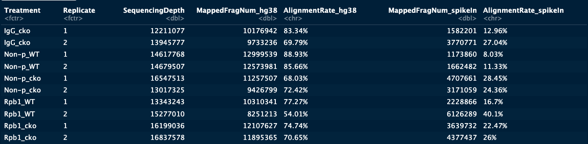
alignSummary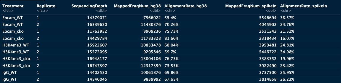
Visualizing the sequencing depth and alignment results.
fig3A = alignResult %>% ggplot(aes(x = Treatment, y = SequencingDepth/1000000, fill = Treatment)) +
    geom_boxplot() +
    geom_jitter(aes(color = Replicate), position = position_jitter(0.15)) +
    scale_fill_viridis(discrete = TRUE, begin = 0.1, end = 0.9, option = "magma", alpha = 0.8) +
    scale_color_viridis(discrete = TRUE, begin = 0.1, end = 0.9) +
    theme_bw(base_size = 18) +
    ylab("Sequencing Depth per Million") +
    xlab("") +
    ggtitle("A. Sequencing Depth")+
    theme(axis.text.x = element_text(angle = 45,vjust = 1, hjust=1))

fig3B = alignResult %>% ggplot(aes(x = Treatment, y = MappedFragNum_hg38/1000000, fill = Treatment)) +
    geom_boxplot() +
    geom_jitter(aes(color = Replicate), position = position_jitter(0.15)) +
    scale_fill_viridis(discrete = TRUE, begin = 0.1, end = 0.9, option = "magma", alpha = 0.8) +
    scale_color_viridis(discrete = TRUE, begin = 0.1, end = 0.9) +
    theme_bw(base_size = 18) +
    ylab("Mapped Fragments per Million") +
    xlab("") +
    ggtitle("B. Alignable Fragment (hg38)")+
      theme(axis.text.x = element_text(angle = 45,vjust = 1, hjust=1))


fig3C = alignResult %>% ggplot(aes(x = Treatment, y = AlignmentRate_hg38, fill = Treatment)) +
    geom_boxplot() +
    geom_jitter(aes(color = Replicate), position = position_jitter(0.15)) +
    scale_fill_viridis(discrete = TRUE, begin = 0.1, end = 0.9, option = "magma", alpha = 0.8) +
    scale_color_viridis(discrete = TRUE, begin = 0.1, end = 0.9) +
    theme_bw(base_size = 18) +
    ylab("% of Mapped Fragments") +
    xlab("") +
    ggtitle("C. Alignment Rate (hg38)")+
      theme(axis.text.x = element_text(angle = 45,vjust = 1, hjust=1))

fig3D = spikeAlign %>% ggplot(aes(x = Treatment, y = AlignmentRate_spikeIn, fill = Treatment)) +
    geom_boxplot() +
    geom_jitter(aes(color = Replicate), position = position_jitter(0.15)) +
    scale_fill_viridis(discrete = TRUE, begin = 0.1, end = 0.9, option = "magma", alpha = 0.8) +
    scale_color_viridis(discrete = TRUE, begin = 0.1, end = 0.9) +
    theme_bw(base_size = 18) +
    ylab("Spike-in Alignment Rate") +
    xlab("") +
    ggtitle("D. Alignment Rate (E.coli)")+
      theme(axis.text.x = element_text(angle = 45,vjust = 1, hjust=1))


ggarrange(fig3A, fig3B, fig3C, fig3D, ncol = 2, nrow=2, common.legend = TRUE, legend="bottom")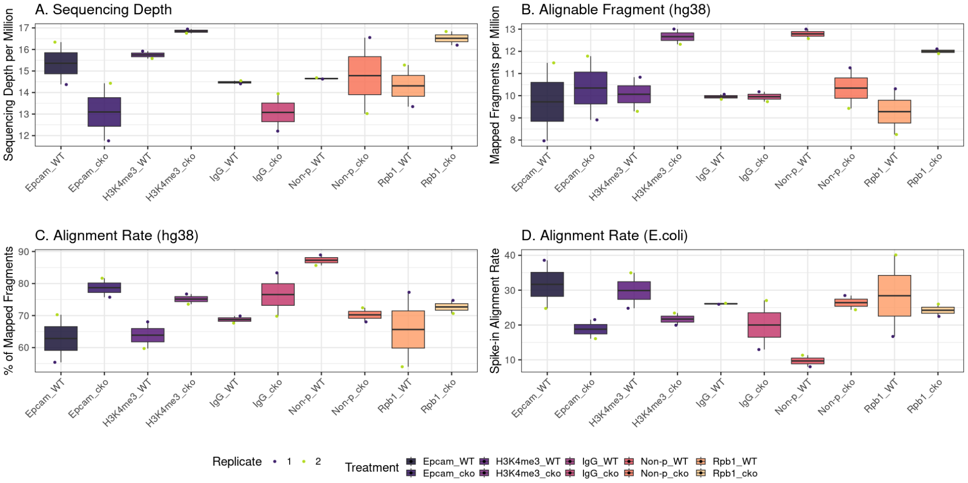
Filtering unmapped and low quality fragments
-q INT only include reads with mapping quality >= INT [0]
for ((i = 0; i < ${#samples[@]}; i+=3)); do
sample_name="${samples[i+2]}"
samtools view -bh -f 3 -F 4 -F 8 -q 10 results/aligned/"$sample_name"_hg38.bam > results/aligned/sorted/"$sample_name"_hg38.step1.bam
done


# for spike-in alignments
for ((i = 0; i < ${#samples[@]}; i+=3)); do
sample_name="${samples[i+2]}"
samtools view -bh -f 3 -F 4 -F 8 -q 10 results/aligned/"$sample_name"_hg38_spikeIn.bam > results/aligned/sorted/"$sample_name"_hg38_spikeIn.step1.bam
done
Sorting BAM
Use picard-2.8.0.jar SortSam
USAGE: SortSam [options]

Documentation: http://broadinstitute.github.io/picard/command-line-overview.html#SortSam

This tool sorts the input SAM or BAM file by coordinate, queryname (QNAME), or some other property of the SAM record.
The SortOrder of a SAM/BAM file is found in the SAM file header tag @HD in the field labeled SO.
For a coordinate sorted SAM/BAM file, read alignments are sorted first by the reference sequence name (RNAME) field
using the reference sequence dictionary (@SQ tag).  Alignments within these subgroups are secondarily sorted using the
left-most mapping position of the read (POS).  Subsequent to this sorting scheme, alignments are listed arbitrarily.

For queryname-sorted alignments, the tool orders records deterministically by queryname field followed by record strand
orientation flag, primary record flag, and secondary alignment flag. This ordering may change in future versions.


Usage example:

java -jar picard.jar SortSam \
I=input.bam \
O=sorted.bam \
SORT_ORDER=coordinate

Version: 2.21.7-SNAPSHOT


Options:

--help
-h                            Displays options specific to this tool.

--stdhelp
-H                            Displays options specific to this tool AND options common to all Picard command line
                              tools.

--version                     Displays program version.

INPUT=File
I=File                        Input BAM or SAM file to sort.  Required.

OUTPUT=File
O=File                        Sorted BAM or SAM output file.  Required.

SORT_ORDER=SortOrder
SO=SortOrder                  Sort order of output file.   Required. Possible values: {
                              queryname (Sorts according to the readname. This will place read-pairs and other derived
                              reads (secondary and supplementary) adjacent to each other. Note that the readnames are
                              compared lexicographically, even though they may include numbers. In paired reads, Read1
                              sorts before Read2.)
                              coordinate (Sorts primarily according to the SEQ and POS fields of the record. The
                              sequence will sorted according to the order in the sequence dictionary, taken from from
                              the header of the file. Within each reference sequence, the reads are sorted by the
                              position. Unmapped reads whose mates are mapped will be placed near their mates. Unmapped
                              read-pairs are placed after all the mapped reads and their mates.)
                              duplicate (Sorts the reads so that duplicates reads are adjacent. Required that the
                              mate-cigar (MC) tag is present. The resulting will be sorted by library, unclipped 5-prime
                              position, orientation, and mate's unclipped 5-prime position.)
                              }
for ((i = 0; i < ${#samples[@]}; i+=3)); do
sample_name="${samples[i+2]}"
java -jar ~/////CUT-RUNTools-2.0-master/install/picard-2.8.0.jar SortSam \
INPUT=results/aligned/sorted/"$sample_name"_hg38.step1.bam \
OUTPUT=results/aligned/sorted/"$sample_name"_hg38.bam \
SORT_ORDER=coordinate \
VALIDATION_STRINGENCY=SILENT \
TMP_DIR=results/log
done
# for spike-in alignments
for ((i = 0; i < ${#samples[@]}; i+=3)); do
sample_name="${samples[i+2]}"
java -jar ~/////CUT-RUNTools-2.0-master/install/picard-2.8.0.jar SortSam \
INPUT=results/aligned/sorted/"$sample_name"_hg38_spikeIn.step1.bam \
OUTPUT=results/aligned/sorted/"$sample_name"_hg38_spikeIn.bam \
SORT_ORDER=coordinate \
VALIDATION_STRINGENCY=SILENT \
TMP_DIR=results/log
doneCreating bam index files (visualize in IGV)
for ((i = 0; i < ${#samples[@]}; i+=3)); do
sample_name="${samples[i+2]}"
samtools index results/aligned/sorted/"$sample_name"_hg38.bam
done
Remove duplicates & visualize duplicate rates
picard-2.8.0.jar MarkDuplicates
USAGE: MarkDuplicates [options]

Documentation: http://broadinstitute.github.io/picard/command-line-overview.html#MarkDuplicates

Identifies duplicate reads.
This tool locates and tags duplicate reads in a BAM or SAM file, where duplicate reads are defined as originating from a
single fragment of DNA.  Duplicates can arise during sample preparation e.g. library construction using PCR.  See also
EstimateLibraryComplexity (https://broadinstitute.github.io/picard/command-line-overview.html#EstimateLibraryComplexity)
for additional notes on PCR duplication artifacts.  Duplicate reads can also result from a single amplification cluster,
incorrectly detected as multiple clusters by the optical sensor of the sequencing instrument.  These duplication
artifacts are referred to as optical duplicates.

The MarkDuplicates tool works by comparing sequences in the 5 prime positions of both reads and read-pairs in a SAM/BAM
file.  An BARCODE_TAG option is available to facilitate duplicate marking using molecular barcodes.  After duplicate
reads are collected, the tool differentiates the primary and duplicate reads using an algorithm that ranks reads by the
sums of their base-quality scores (default method).

The tool's main output is a new SAM or BAM file, in which duplicates have been identified in the SAM flags field for
each read.  Duplicates are marked with the hexadecimal value of 0x0400, which corresponds to a decimal value of 1024.
If you are not familiar with this type of annotation, please see the following blog post
(https://www.broadinstitute.org/gatk/blog?id=7019) for additional information.

Although the bitwise flag annotation indicates whether a read was marked as a duplicate, it does not identify the type
of duplicate.  To do this, a new tag called the duplicate type (DT) tag was recently added as an optional output in  the
'optional field' section of a SAM/BAM file.  Invoking the TAGGING_POLICY option, you can instruct the program to mark
all the duplicates (All), only the optical duplicates (OpticalOnly), or no duplicates (DontTag).  The records within the
output of a SAM/BAM file will have values for the 'DT' tag (depending on the invoked TAGGING_POLICY), as either
library/PCR-generated duplicates (LB), or sequencing-platform artifact duplicates (SQ).  This tool uses the
READ_NAME_REGEX and the OPTICAL_DUPLICATE_PIXEL_DISTANCE options as the primary methods to identify and differentiate
duplicate types.  Set READ_NAME_REGEX to null to skip optical duplicate detection, e.g. for RNA-seq or other data where
duplicate sets are extremely large and estimating library complexity is not an aim.  Note that without optical duplicate
counts, library size estimation will be inaccurate.

MarkDuplicates also produces a metrics file indicating the numbers of duplicates for both single- and paired-end reads.

The program can take either coordinate-sorted or query-sorted inputs, however the behavior is slightly different.  When
the input is coordinate-sorted, unmapped mates of mapped records and supplementary/secondary alignments are not marked
as duplicates.  However, when the input is query-sorted (actually query-grouped), then unmapped mates and
secondary/supplementary reads are not excluded from the duplication test and can be marked as duplicate reads.

If desired, duplicates can be removed using the REMOVE_DUPLICATE and REMOVE_SEQUENCING_DUPLICATES options.

Usage example:

java -jar picard.jar MarkDuplicates \
I=input.bam \
O=marked_duplicates.bam \
M=marked_dup_metrics.txt
Please see MarkDuplicates (http://broadinstitute.github.io/picard/picard-metric-definitions.html#DuplicationMetrics) for
detailed explanations of the output metrics.

Version: 2.21.7-SNAPSHOT


Options:

--help
-h                            Displays options specific to this tool.

--stdhelp
-H                            Displays options specific to this tool AND options common to all Picard command line
                              tools.

--version                     Displays program version.

MAX_SEQUENCES_FOR_DISK_READ_ENDS_MAP=Integer
MAX_SEQS=Integer              This option is obsolete. ReadEnds will always be spilled to disk.  Default value: 50000.
                              This option can be set to 'null' to clear the default value.

MAX_FILE_HANDLES_FOR_READ_ENDS_MAP=Integer
MAX_FILE_HANDLES=Integer      Maximum number of file handles to keep open when spilling read ends to disk. Set this
                              number a little lower than the per-process maximum number of file that may be open. This
                              number can be found by executing the 'ulimit -n' command on a Unix system.  Default value:
                              8000. This option can be set to 'null' to clear the default value.

SORTING_COLLECTION_SIZE_RATIO=Double
                              This number, plus the maximum RAM available to the JVM, determine the memory footprint
                              used by some of the sorting collections.  If you are running out of memory, try reducing
                              this number.  Default value: 0.25. This option can be set to 'null' to clear the default
                              value.

BARCODE_TAG=String            Barcode SAM tag (ex. BC for 10X Genomics)  Default value: null.

READ_ONE_BARCODE_TAG=String   Read one barcode SAM tag (ex. BX for 10X Genomics)  Default value: null.

READ_TWO_BARCODE_TAG=String   Read two barcode SAM tag (ex. BX for 10X Genomics)  Default value: null.

TAG_DUPLICATE_SET_MEMBERS=Boolean
                              If a read appears in a duplicate set, add two tags. The first tag, DUPLICATE_SET_SIZE_TAG
                              (DS), indicates the size of the duplicate set. The smallest possible DS value is 2 which
                              occurs when two reads map to the same portion of the reference only one of which is marked
                              as duplicate. The second tag, DUPLICATE_SET_INDEX_TAG (DI), represents a unique identifier
                              for the duplicate set to which the record belongs. This identifier is the index-in-file of
                              the representative read that was selected out of the duplicate set.  Default value: false.
                              This option can be set to 'null' to clear the default value. Possible values: {true,
                              false}

REMOVE_SEQUENCING_DUPLICATES=Boolean
                              If true remove 'optical' duplicates and other duplicates that appear to have arisen from
                              the sequencing process instead of the library preparation process, even if
                              REMOVE_DUPLICATES is false. If REMOVE_DUPLICATES is true, all duplicates are removed and
                              this option is ignored.  Default value: false. This option can be set to 'null' to clear
                              the default value. Possible values: {true, false}

TAGGING_POLICY=DuplicateTaggingPolicy
                              Determines how duplicate types are recorded in the DT optional attribute.  Default value:
                              DontTag. This option can be set to 'null' to clear the default value. Possible values:
                              {DontTag, OpticalOnly, All}

CLEAR_DT=Boolean              Clear DT tag from input SAM records. Should be set to false if input SAM doesn't have this
                              tag.  Default true  Default value: true. This option can be set to 'null' to clear the
                              default value. Possible values: {true, false}

DUPLEX_UMI=Boolean            Treat UMIs as being duplex stranded.  This option requires that the UMI consist of two
                              equal length strings that are separated by a hyphen (e.g. 'ATC-GTC'). Reads are considered
                              duplicates if, in addition to standard definition, have identical normalized UMIs.  A UMI
                              from the 'bottom' strand is normalized by swapping its content around the hyphen (eg.
                              ATC-GTC becomes GTC-ATC).  A UMI from the 'top' strand is already normalized as it is.
                              Both reads from a read pair considered top strand if the read 1 unclipped 5' coordinate is
                              less than the read 2 unclipped 5' coordinate. All chimeric reads and read fragments are
                              treated as having come from the top strand. With this option is it required that the
                              BARCODE_TAG hold non-normalized UMIs. Default false.  Default value: false. This option
                              can be set to 'null' to clear the default value. Possible values: {true, false}

MOLECULAR_IDENTIFIER_TAG=String
                              SAM tag to uniquely identify the molecule from which a read was derived.  Use of this
                              option requires that the BARCODE_TAG option be set to a non null value.  Default null.
                              Default value: null.

INPUT=String
I=String                      One or more input SAM or BAM files to analyze. Must be coordinate sorted.  Default value:
                              null. This option may be specified 0 or more times.

OUTPUT=File
O=File                        The output file to write marked records to  Required.

METRICS_FILE=File
M=File                        File to write duplication metrics to  Required.

REMOVE_DUPLICATES=Boolean     If true do not write duplicates to the output file instead of writing them with
                              appropriate flags set.  Default value: false. This option can be set to 'null' to clear
                              the default value. Possible values: {true, false}

ASSUME_SORTED=Boolean
AS=Boolean                    If true, assume that the input file is coordinate sorted even if the header says
                              otherwise. Deprecated, used ASSUME_SORT_ORDER=coordinate instead.  Default value: false.
                              This option can be set to 'null' to clear the default value. Possible values: {true,
                              false}  Cannot be used in conjuction with option(s) ASSUME_SORT_ORDER (ASO)

ASSUME_SORT_ORDER=SortOrder
ASO=SortOrder                 If not null, assume that the input file has this order even if the header says otherwise.
                              Default value: null. Possible values: {unsorted, queryname, coordinate, duplicate,
                              unknown}  Cannot be used in conjuction with option(s) ASSUME_SORTED (AS)

DUPLICATE_SCORING_STRATEGY=ScoringStrategy
DS=ScoringStrategy            The scoring strategy for choosing the non-duplicate among candidates.  Default value:
                              SUM_OF_BASE_QUALITIES. This option can be set to 'null' to clear the default value.
                              Possible values: {SUM_OF_BASE_QUALITIES, TOTAL_MAPPED_REFERENCE_LENGTH, RANDOM}

PROGRAM_RECORD_ID=String
PG=String                     The program record ID for the @PG record(s) created by this program. Set to null to
                              disable PG record creation.  This string may have a suffix appended to avoid collision
                              with other program record IDs.  Default value: MarkDuplicates. This option can be set to
                              'null' to clear the default value.

PROGRAM_GROUP_VERSION=String
PG_VERSION=String             Value of VN tag of PG record to be created. If not specified, the version will be detected
                              automatically.  Default value: null.

PROGRAM_GROUP_COMMAND_LINE=String
PG_COMMAND=String             Value of CL tag of PG record to be created. If not supplied the command line will be
                              detected automatically.  Default value: null.

PROGRAM_GROUP_NAME=String
PG_NAME=String                Value of PN tag of PG record to be created.  Default value: MarkDuplicates. This option
                              can be set to 'null' to clear the default value.

COMMENT=String
CO=String                     Comment(s) to include in the output file's header.  Default value: null. This option may
                              be specified 0 or more times.

READ_NAME_REGEX=String        MarkDuplicates can use the tile and cluster positions to estimate the rate of optical
                              duplication in addition to the dominant source of duplication, PCR, to provide a more
                              accurate estimation of library size. By default (with no READ_NAME_REGEX specified),
                              MarkDuplicates will attempt to extract coordinates using a split on ':' (see Note below).
                              Set READ_NAME_REGEX to 'null' to disable optical duplicate detection. Note that without
                              optical duplicate counts, library size estimation will be less accurate. If the read name
                              does not follow a standard Illumina colon-separation convention, but does contain tile and
                              x,y coordinates, a regular expression can be specified to extract three variables:
                              tile/region, x coordinate and y coordinate from a read name. The regular expression must
                              contain three capture groups for the three variables, in order. It must match the entire
                              read name.   e.g. if field names were separated by semi-colon (';') this example regex
                              could be specified      (?:.*;)?([0-9]+)[^;]*;([0-9]+)[^;]*;([0-9]+)[^;]*$ Note that if no
                              READ_NAME_REGEX is specified, the read name is split on ':'.   For 5 element names, the
                              3rd, 4th and 5th elements are assumed to be tile, x and y values.   For 7 element names
                              (CASAVA 1.8), the 5th, 6th, and 7th elements are assumed to be tile, x and y values.
                              Default value: <optimized capture of last three ':' separated fields as numeric values>.
                              This option can be set to 'null' to clear the default value.

OPTICAL_DUPLICATE_PIXEL_DISTANCE=Integer
                              The maximum offset between two duplicate clusters in order to consider them optical
                              duplicates. The default is appropriate for unpatterned versions of the Illumina platform.
                              For the patterned flowcell models, 2500 is moreappropriate. For other platforms and
                              models, users should experiment to find what works best.  Default value: 100. This option
                              can be set to 'null' to clear the default value.

MAX_OPTICAL_DUPLICATE_SET_SIZE=Long
                              This number is the maximum size of a set of duplicate reads for which we will attempt to
                              determine which are optical duplicates.  Please be aware that if you raise this value too
                              high and do encounter a very large set of duplicate reads, it will severely affect the
                              runtime of this tool.  To completely disable this check, set the value to -1.  Default
                              value: 300000. This option can be set to 'null' to clear the default value.
for ((i = 0; i < ${#samples[@]}; i+=3)); do
sample_name="${samples[i+2]}"
## remove duplicates
java -jar ~/////CUT-RUNTools-2.0-master/install/picard-2.8.0.jar MarkDuplicates \
INPUT=results/aligned/sorted/"$sample_name"_hg38.bam \
OUTPUT=results/aligned/dedup/"$sample_name"_hg38.bam \
VALIDATION_STRINGENCY=SILENT \
TMP_DIR=results/log \
REMOVE_DUPLICATES=true \
METRICS_FILE=results/log/"$sample_name"_hg38.dedup
done→ Access boxplot figure for the duplication rate in R
projPath = "~////01_trimmed_reads/results"


dupResult = c()
for(hist in sampleList){
  dupRes = read.table(paste0(projPath, "/log/", hist, "_hg38.dedup"), header = TRUE, fill = TRUE)

  histInfo = strsplit(hist, "_")[[1]]

  dupResult = data.frame(Treatment = paste0(histInfo[1],"_",histInfo[2]),
                         Replicate = histInfo[3],
                         MappedFragNum_filtered = dupRes$READ_PAIRS_EXAMINED[1] %>%
                           as.character %>%
                           as.numeric,
                         DuplicationRate = dupRes$PERCENT_DUPLICATION[1] %>%
                           as.character %>%
                           as.numeric * 100,
                         EstimatedLibrarySize = dupRes$ESTIMATED_LIBRARY_SIZE[1] %>%
                           as.character %>%
                           as.numeric) %>%
  mutate(UniqueFragNum = MappedFragNum_filtered * (1-DuplicationRate/100))  %>%
    rbind(dupResult, .)
}
dupResult$Treatment = factor(dupResult$Treatment, levels = histList)

alignDupSummary = left_join(alignResult,
                            dupResult,
                            by = c("Treatment", "Replicate")) %>%
  mutate(DuplicationRate = paste0(DuplicationRate, "%"))

alignDupSummary
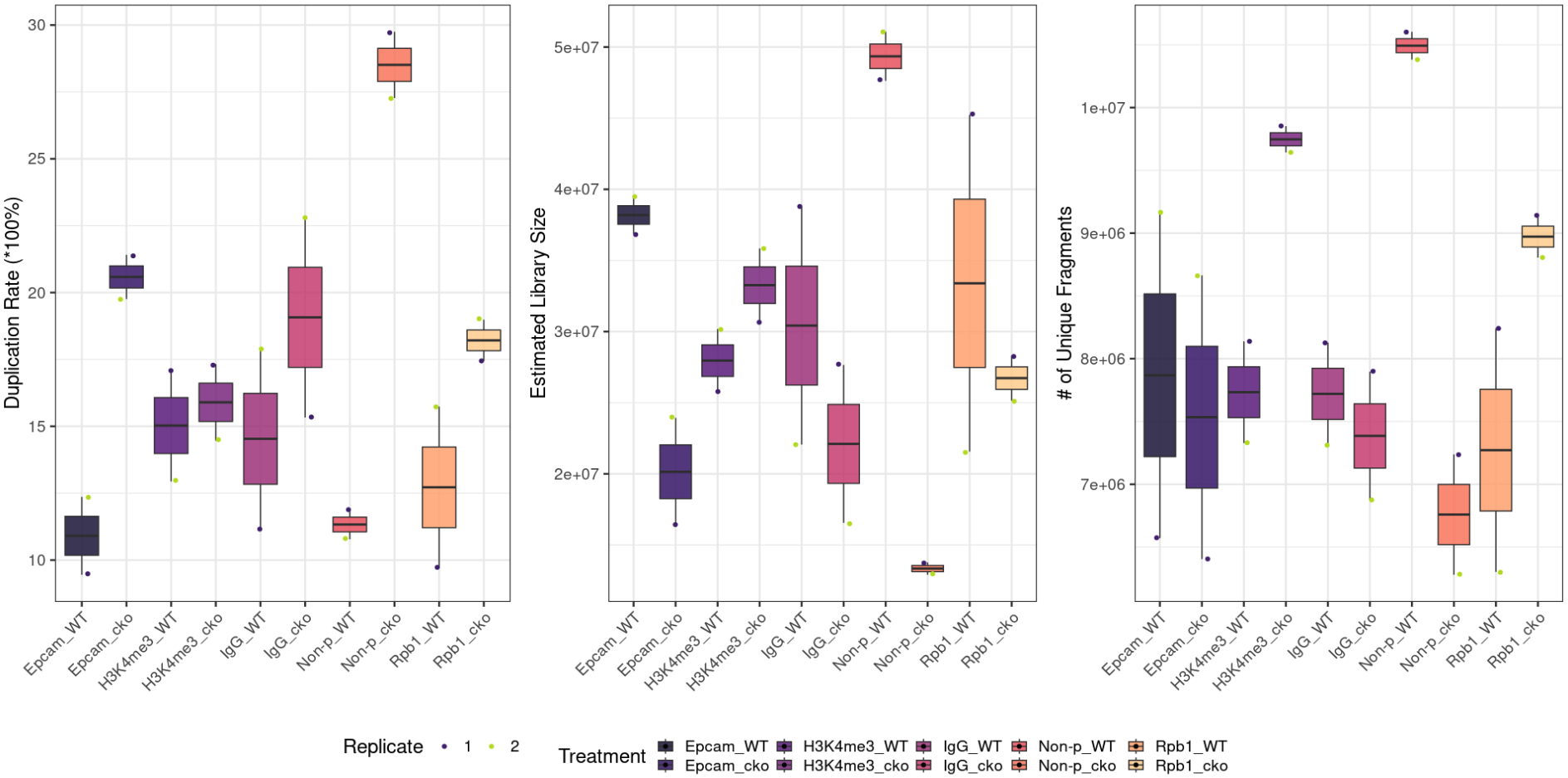
fig4A = dupResult %>% ggplot(aes(x = Treatment, y = DuplicationRate, fill = Treatment)) +
geom_boxplot() +
geom_jitter(aes(color = Replicate), position = position_jitter(0.15)) +
scale_fill_viridis(discrete = TRUE, begin = 0.1, end = 0.9, option = "magma", alpha = 0.8) +
scale_color_viridis(discrete = TRUE, begin = 0.1, end = 0.9) +
theme_bw(base_size = 18) +
ylab("Duplication Rate (*100%)") +
xlab("")+
theme(axis.text.x = element_text(angle = 45,vjust = 1, hjust=1))
fig4B = dupResult %>% ggplot(aes(x = Treatment, y = EstimatedLibrarySize, fill = Treatment)) +
geom_boxplot() +
geom_jitter(aes(color = Replicate), position = position_jitter(0.15)) +
scale_fill_viridis(discrete = TRUE, begin = 0.1, end = 0.9, option = "magma", alpha = 0.8) +
scale_color_viridis(discrete = TRUE, begin = 0.1, end = 0.9) +
theme_bw(base_size = 18) +
ylab("Estimated Library Size") +
xlab("")+
theme(axis.text.x = element_text(angle = 45,vjust = 1, hjust=1))
fig4C = dupResult %>% ggplot(aes(x = Treatment, y = UniqueFragNum, fill = Treatment)) +
geom_boxplot() +
geom_jitter(aes(color = Replicate), position = position_jitter(0.15)) +
scale_fill_viridis(discrete = TRUE, begin = 0.1, end = 0.9, option = "magma", alpha = 0.8) +
scale_color_viridis(discrete = TRUE, begin = 0.1, end = 0.9) +
theme_bw(base_size = 18) +
ylab("# of Unique Fragments") +
xlab("")+
theme(axis.text.x = element_text(angle = 45,vjust = 1, hjust=1))
ggarrange(fig4A, fig4B, fig4C, ncol = 3, common.legend = TRUE, legend="bottom")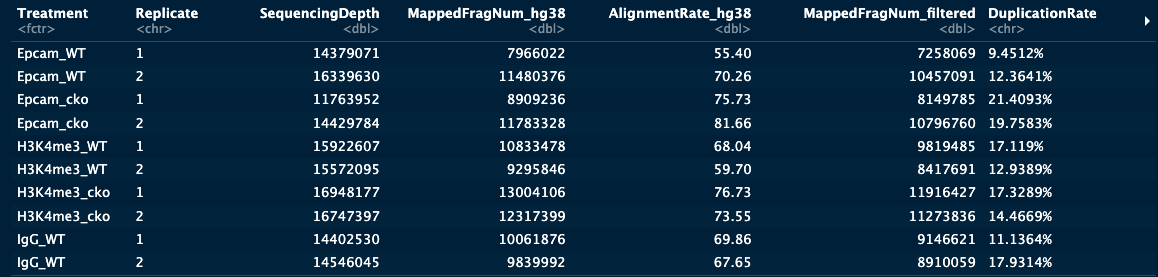
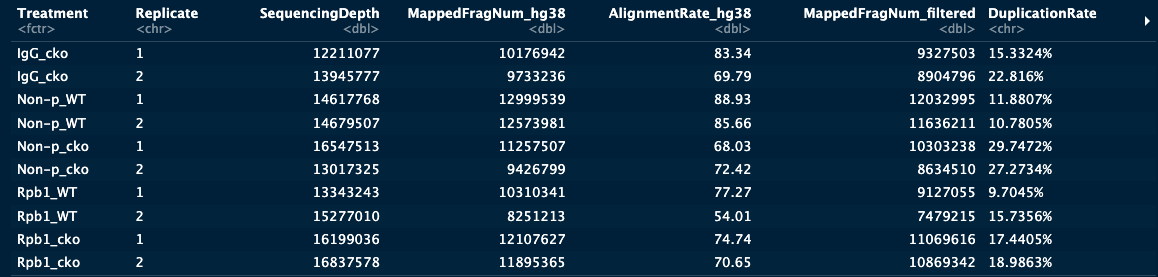
Here I did not remove duplicates
so I use results/aligned/sorted/*_hg38.bam as my BAM files to perform downstream analysis
Assess mapped fragment size distribution
mkdir results/aligned/sorted/fragmentLen

for ((i = 0; i < ${#samples[@]}; i+=3)); do
sample_name="${samples[i+2]}"
## Extract the 9th column from the alignment sam file which is the fragment length
samtools view -F 0x04 results/aligned/sorted/"$sample_name"_hg38.bam | awk -F'\t' 'function abs(x){return ((x < 0.0) ? -x : x)} {print abs($9)}' | sort | uniq -c | awk -v OFS="\t" '{print $2, $1/2}' > results/aligned/sorted/fragmentLen/"$sample_name"_hg38_fragmentLen.txt
done
Assess mapped fragment size distribution in R
fragLen = c()

for(hist in sampleList){

  histInfo = strsplit(hist, "_")[[1]]
  fragLen = read.table(paste0(projPath, "/aligned/sorted/fragmentLen/", hist, "_hg38_fragmentLen.txt"), header = FALSE) %>%
    mutate(fragLen = V1 %>% as.numeric,
           fragCount = V2 %>% as.numeric,
           Treatment = paste0(histInfo[1],"_",histInfo[2]),
           Replicate = histInfo[3],
           sampleInfo = hist) %>% rbind(fragLen, .)
}

fragLen$sampleInfo = factor(fragLen$sampleInfo, levels = sampleList)
fragLen$Treatment = factor(fragLen$Treatment, levels = histList)


fig5B = fragLen %>% ggplot(aes(x = fragLen,
                               y = fragCount,
                               color = Treatment,
                               group = sampleInfo,
                               linetype = Replicate)) +
  geom_line(linewidth = 1) +
  scale_color_viridis(discrete = TRUE, begin = 0.1, end = 0.9, option = "magma") +
  theme_bw(base_size = 20) +
  xlab("Fragment Length") +
  ylab("Count") +
  coord_cartesian(xlim = c(0, 500))

fig5B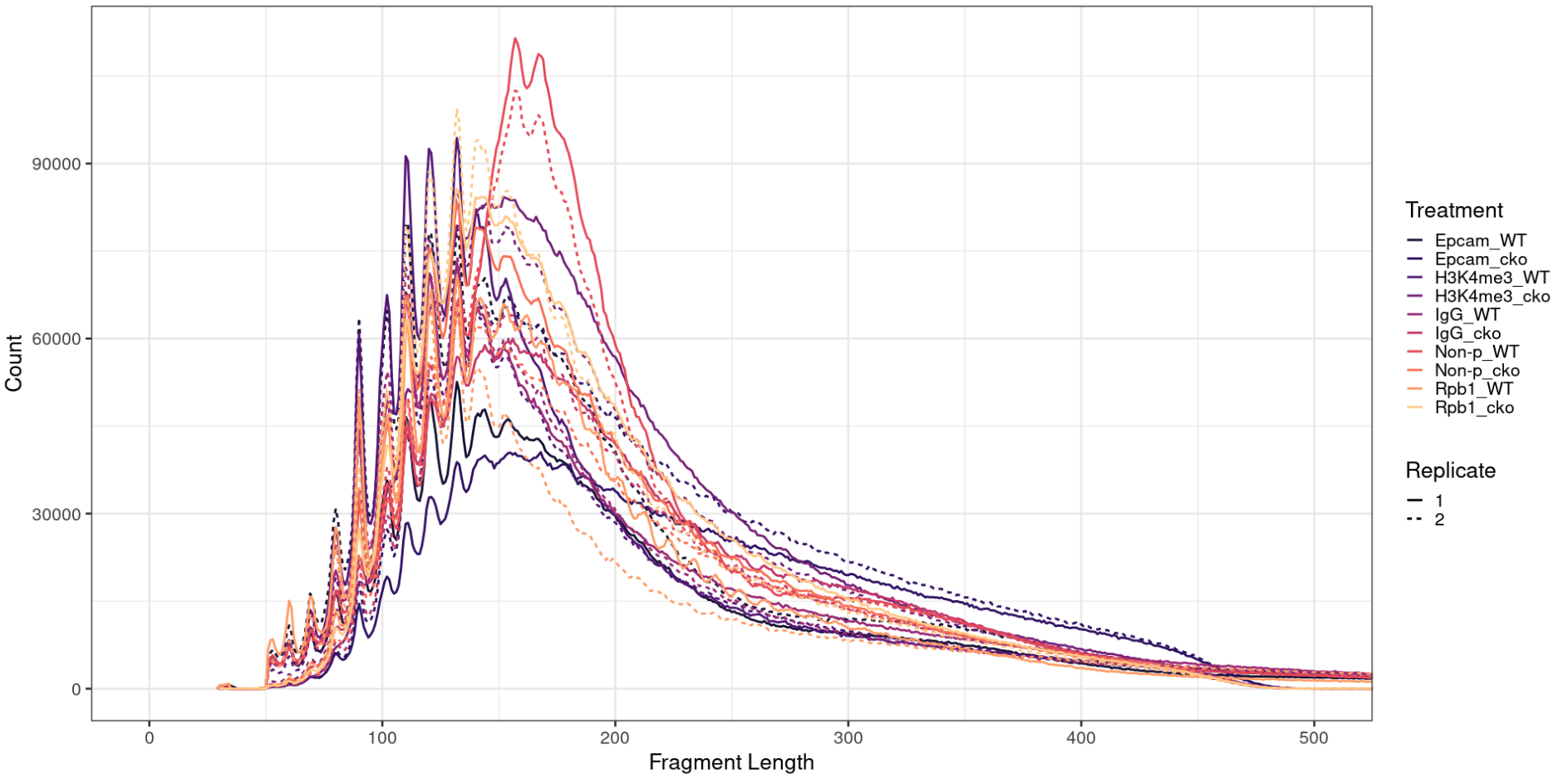
Spike-in calibration (Calibration, generate bedgraph files for SEACR)
In the formular scale_factor = C / (fragments mapped to E. coli genome), if we make C too small (supposed to be 10000 according to the original pipeline) → leads to most coverage <1 → being filtered out → can not call any peak with SEACR top0.01 threshold.
In the original pipeline, the spike-in mapped fragments before filtering is 235 - 79123. Here we have 1173860 - 6126289.
So here we set the C to 20,000,000.
https://github.com/mbassalbioinformatics/CnRAP/issues/2 The author of CnRAP suggested that scale_factor should be something between 5 to 20。
***→ ***🔑 We suggested that we set the value of C to the lowest spike-in aligned fragments in the future.
for ((i = 0; i < ${#samples[@]}; i+=3)); do

sample_name="${samples[i+2]}"
bam_file=results/aligned/sorted/"$sample_name"_hg38.bam

# calculate scale factor from spikeIn.bam
seqDepthDouble=`samtools view -F 0x04 results/aligned/sorted/"$sample_name"_hg38_spikeIn.bam | wc -l`
seqDepth=$((seqDepthDouble/2))
echo $seqDepth > results/aligned/sorted/"$sample_name"_bowtie2_spikeIn.seqDepth

if [[ "$seqDepth" -gt "1" ]]; then
scale_factor=`echo "20000000 / $seqDepth" | bc -l`
echo "Scaling factor for $sample_name is: $scale_factor!"

# spike-in normalization
bedtools genomecov -bg -scale $scale_factor \
-ibam $bam_file > results/peakcalling/seacr/"$sample_name"_hg38.normalized_20m.bedgraph

python ~/////CUT-RUNTools-2.0-master/install/change.bdg.py \
results/peakcalling/seacr/"$sample_name"_hg38.normalized_20m.bedgraph > results/peakcalling/seacr/"$sample_name"_hg38.normalized_20m.integer.bedgraph
fi

done
Scaling factor for Epcam_WT_1 is: 3.65999924604015531572!
Scaling factor for Epcam_WT_2 is: 5.01526772878334870930!
Scaling factor for Epcam_cko_1 is: 8.01943912042791727146!
Scaling factor for Epcam_cko_2 is: 8.75496132714707765957!
Scaling factor for H3K4me3_WT_1 is: 5.13816262387467815833!
Scaling factor for H3K4me3_WT_2 is: 3.72646481276284386652!
Scaling factor for H3K4me3_cko_1 is: 5.99820473732211948963!
Scaling factor for H3K4me3_cko_2 is: 5.17442602032566285044!
Scaling factor for IgG_WT_1 is: 5.43100599338666400185!
Scaling factor for IgG_WT_2 is: 5.32262138038459665308!
Scaling factor for IgG_cko_1 is: 12.82045529282881422967!
Scaling factor for IgG_cko_2 is: 5.38291210700368002786!
Scaling factor for Non-p_WT_1 is: 17.29441053298779101088!
Scaling factor for Non-p_WT_2 is: 12.21556813080430354465!
Scaling factor for Non-p_cko_1 is: 4.31064490049630610061!
Scaling factor for Non-p_cko_2 is: 6.39990579338672134746!
Scaling factor for Rpb1_WT_1 is: 9.10926425838974624778!
Scaling factor for Rpb1_WT_2 is: 3.31232381542605510348!
Scaling factor for Rpb1_cko_1 is: 5.57522992248200315781!
Scaling factor for Rpb1_cko_2 is: 4.63681132049663031329!Scaling factor in R
scaleFactor = c()
multiplier = 20000000
for(hist in sampleList){
  spikeDepth = read.table(paste0(projPath, "/aligned/sorted/", hist, "_bowtie2_spikeIn.seqDepth"), header = FALSE, fill = TRUE)$V1[1]

  histInfo = strsplit(hist, "_")[[1]]
  scaleFactor = data.frame(scaleFactor = multiplier/spikeDepth,
													 Treatment = paste0(histInfo[1],"_",histInfo[2]),
													 Replicate = histInfo[3])  %>% rbind(scaleFactor, .)
}

scaleFactor$Treatment = factor(scaleFactor$Treatment, levels = histList)
left_join(alignDupSummary, scaleFactor, by = c("Treatment", "Replicate"))
fig6A = scaleFactor %>% ggplot(aes(x = Treatment, y = scaleFactor, fill = Treatment)) +
geom_boxplot() +
geom_jitter(aes(color = Replicate), position = position_jitter(0.15)) +
scale_fill_viridis(discrete = TRUE, begin = 0.1, end = 0.9, option = "magma", alpha = 0.8) +
scale_color_viridis(discrete = TRUE, begin = 0.1, end = 0.9) +
theme_bw(base_size = 20) +
ylab("Spike-in Scalling Factor") +
xlab("")+
theme(axis.text.x = element_text(angle = 45,vjust = 1, hjust=1))
normDepth = inner_join(scaleFactor, alignDupSummary, by = c("Treatment", "Replicate")) %>% mutate(normDepth = MappedFragNum_filtered * scaleFactor)
fig6B = normDepth %>% ggplot(aes(x = Treatment, y = normDepth, fill = Treatment)) +
geom_boxplot() +
geom_jitter(aes(color = Replicate), position = position_jitter(0.15)) +
scale_fill_viridis(discrete = TRUE, begin = 0.1, end = 0.9, option = "magma", alpha = 0.8) +
scale_color_viridis(discrete = TRUE, begin = 0.1, end = 0.9) +
theme_bw(base_size = 20) +
ylab("Normalization Fragment Count") +
xlab("") +
coord_cartesian(ylim = c(1000000, 210000000))+
theme(axis.text.x = element_text(angle = 45,vjust = 1, hjust=1))
ggarrange(fig6A, fig6B, ncol = 2, common.legend = TRUE, legend="bottom")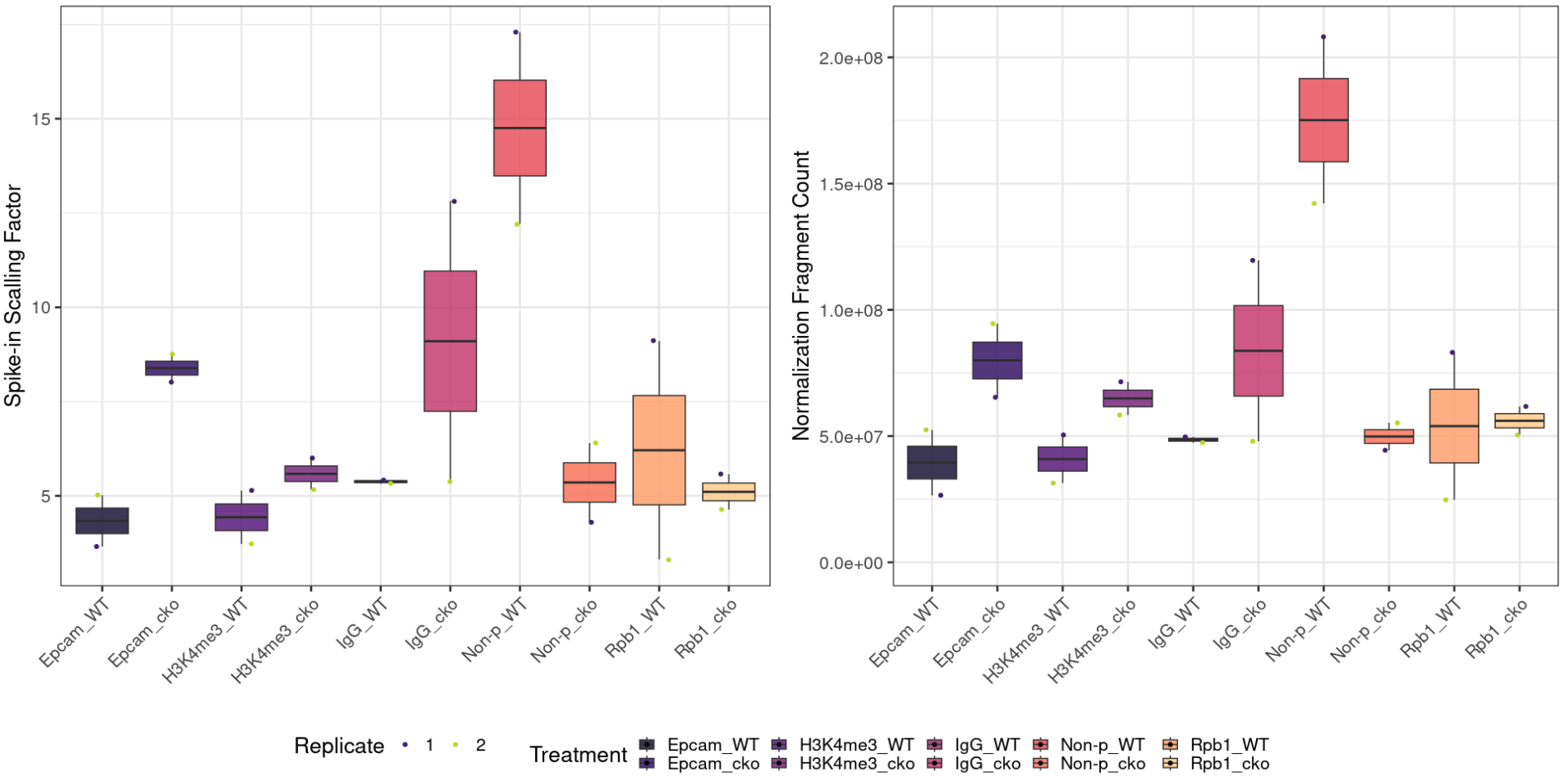
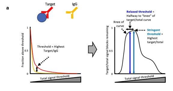
There are 2 modes of SEACR (see here), here we compare the results of them:
- without IgG control + top0.01
- with IgG control threshold n (between 0 and 1): returns the top n fraction of peaks based on total signal within peaks → we set to 0.01
In addition there are stringent and relaxed mode (Here we use stringent mode)
“relaxed” uses a total signal threshold between the knee and peak of the total signal curve, and corresponds to the “relaxed” mode described in the text, whereas “stringent” uses the peak of the curve, and corresponds to “stringent” mode.
Peak calling using SEACR “non stringent” + “top 0.01”
Rscriptbin="///////CondaEnv/CUTRUNTools/bin"


for ((i = 0; i < ${#samples[@]}; i+=3)); do
sample_name="${samples[i+2]}"

SEACR_1.3.sh \
results/peakcalling/seacr/"$sample_name"_hg38.normalized_20m.integer.bedgraph \
0.01 non stringent \
results/peakcalling/seacr/"$sample_name"_hg38.normalized_20m_treat_top0.01 \
$Rscriptbin

sort-bed results/peakcalling/seacr/"$sample_name"_hg38.normalized_20m_treat_top0.01.stringent.bed > results/peakcalling/seacr/"$sample_name"_hg38.normalized_20m_treat_top0.01.stringent.sort.bed

done
We can call peaks on all samples.
Peak calling using SEACR “non stringent” + “IgG control”
samples_WT1=(
  "Epcam_WT1_1.paired.fastq.gz" "Epcam_WT1_2.paired.fastq.gz" "Epcam_WT_1"
  "H3K4me3_WT1_1.paired.fastq.gz" "H3K4me3_WT1_2.paired.fastq.gz" "H3K4me3_WT_1"
  "Non-p_WT1_1.paired.fastq.gz" "Non-p_WT1_2.paired.fastq.gz" "Non-p_WT_1"
  "Rpb1_WT1_1.paired.fastq.gz" "Rpb1_WT1_2.paired.fastq.gz" "Rpb1_WT_1"
)


samples_WT2=(
  "Epcam_WT2_1.paired.fastq.gz" "Epcam_WT2_2.paired.fastq.gz" "Epcam_WT_2"
  "H3K4me3_WT2_1.paired.fastq.gz" "H3K4me3_WT2_2.paired.fastq.gz" "H3K4me3_WT_2"
  "Non-p_WT2_1.paired.fastq.gz" "Non-p_WT2_2.paired.fastq.gz" "Non-p_WT_2"
  "Rpb1_WT2_1.paired.fastq.gz" "Rpb1_WT2_2.paired.fastq.gz" "Rpb1_WT_2"
)


samples_cko1=(
  "Epcam_cko1_1.paired.fastq.gz" "Epcam_cko1_2.paired.fastq.gz" "Epcam_cko_1"
  "H3K4me3_cko1_1.paired.fastq.gz" "H3K4me3_cko1_2.paired.fastq.gz" "H3K4me3_cko_1"
  "Non-p_cko1_1.paired.fastq.gz" "Non-p_cko1_2.paired.fastq.gz" "Non-p_cko_1"
  "Rpb1_cko1_1.paired.fastq.gz" "Rpb1_cko1_2.paired.fastq.gz" "Rpb1_cko_1"
)


samples_cko2=(
  "Epcam_cko2_1.paired.fastq.gz" "Epcam_cko2_2.paired.fastq.gz" "Epcam_cko_2"
  "H3K4me3_cko2_1.paired.fastq.gz" "H3K4me3_cko2_2.paired.fastq.gz" "H3K4me3_cko_2"
  "Non-p_cko2_1.paired.fastq.gz" "Non-p_cko2_2.paired.fastq.gz" "Non-p_cko_2"
  "Rpb1_cko2_1.paired.fastq.gz" "Rpb1_cko2_2.paired.fastq.gz" "Rpb1_cko_2"
)


Rscriptbin="/data/core/jordan/CondaEnv/CUTRUNTools/bin"

----------
# WT1 sample, use IgG WT1 as control

for ((i = 0; i < ${#samples_WT1[@]}; i+=3)); do
sample_name="${samples_WT1[i+2]}"

SEACR_1.3.sh \
results/peakcalling/seacr/"$sample_name"_hg38.normalized_20m.integer.bedgraph \
results/peakcalling/seacr/IgG_WT_1_hg38.normalized_20m.integer.bedgraph \
non stringent \
results/peakcalling/seacr/"$sample_name"_hg38.normalized_20m_treat_control \
$Rscriptbin

sort-bed results/peakcalling/seacr/"$sample_name"_hg38.normalized_20m_treat_control.stringent.bed > results/peakcalling/seacr/"$sample_name"_hg38.normalized_20m_treat_control.stringent.sort.bed
done


# WT2 sample, use IgG WT2 as control

for ((i = 0; i < ${#samples_WT2[@]}; i+=3)); do
sample_name="${samples_WT2[i+2]}"

SEACR_1.3.sh \
results/peakcalling/seacr/"$sample_name"_hg38.normalized_20m.integer.bedgraph \
results/peakcalling/seacr/IgG_WT_2_hg38.normalized_20m.integer.bedgraph \
non stringent \
results/peakcalling/seacr/"$sample_name"_hg38.normalized_20m_treat_control \
$Rscriptbin

sort-bed results/peakcalling/seacr/"$sample_name"_hg38.normalized_20m_treat_control.stringent.bed > results/peakcalling/seacr/"$sample_name"_hg38.normalized_20m_treat_control.stringent.sort.bed
done


# cko1 sample, use IgG cko1 as control

for ((i = 0; i < ${#samples_cko1[@]}; i+=3)); do
sample_name="${samples_cko1[i+2]}"

SEACR_1.3.sh \
results/peakcalling/seacr/"$sample_name"_hg38.normalized_20m.integer.bedgraph \
results/peakcalling/seacr/IgG_cko_1_hg38.normalized_20m.integer.bedgraph \
non stringent \
results/peakcalling/seacr/"$sample_name"_hg38.normalized_20m_treat_control \
$Rscriptbin

sort-bed results/peakcalling/seacr/"$sample_name"_hg38.normalized_20m_treat_control.stringent.bed > results/peakcalling/seacr/"$sample_name"_hg38.normalized_20m_treat_control.stringent.sort.bed
done


# cko2 sample, use IgG cko2 as control

for ((i = 0; i < ${#samples_cko2[@]}; i+=3)); do
sample_name="${samples_cko2[i+2]}"

SEACR_1.3.sh \
results/peakcalling/seacr/"$sample_name"_hg38.normalized_20m.integer.bedgraph \
results/peakcalling/seacr/IgG_cko_2_hg38.normalized_20m.integer.bedgraph \
non stringent \
results/peakcalling/seacr/"$sample_name"_hg38.normalized_20m_treat_control \
$Rscriptbin

sort-bed results/peakcalling/seacr/"$sample_name"_hg38.normalized_20m_treat_control.stringent.bed > results/peakcalling/seacr/"$sample_name"_hg38.normalized_20m_treat_control.stringent.sort.bed
done
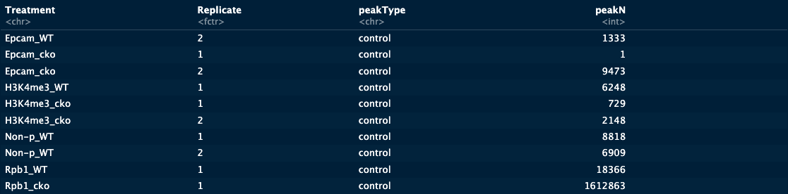
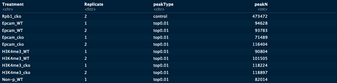
Eventually we fail to call peaks on many samples with IgG control
- Epcam_WT_1
- H3K4me3_WT_2
- Non-p_cko_1
- Non-p_cko_2
- Rpb1_WT_2
Calculate peaks in R
Peak Number
projPath = "~/////01_trimmed_reads/results"

peakN = c()
peakWidth = c()
peakType = c("control", "top0.01")
Sample = c("Epcam_WT","Epcam_cko",
          "H3K4me3_WT","H3K4me3_cko",
          "Non-p_WT","Non-p_cko",
          "Rpb1_WT","Rpb1_cko")

      for(type in peakType){
        for (sample in Sample) {
          for (rep in c(1,2)) {
              file_path = paste0(projPath,
                                 "/peakcalling/seacr/",
                                 sample, "_", rep,
                                 "_hg38.normalized_20m_treat_", type, ".stringent.sort.bed")

              # Check if the file exists and has a non-zero size before reading
              if (file.exists(file_path) && file.info(file_path)$size > 0) {

               peakInfo = read.table(file_path, header = FALSE, fill = TRUE)  %>%
                          mutate(width = abs(V3-V2))
               peakN <- rbind(peakN,
                              data.frame(peakN = nrow(peakInfo),
                                         peakType = type,
                                         Treatment = sample,
                                         Replicate = rep))
               peakWidth = rbind(peakWidth,
                                 data.frame(width = peakInfo$width,
                                 peakType = type,
                                 Treatment = sample,
                                 Replicate = rep))

                                                                           } else {
               print(paste0("The file ", file_path, " does not exist or contains no peaks."))}

                             }
                              }
                           }

peakN$Replicate <- factor(peakN$Replicate, levels = c(1,2))

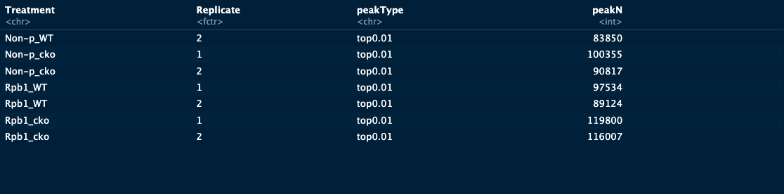
peakN %>%
dplyr::select(Treatment, Replicate, peakType, peakN)[1] "The file ~/////01_trimmed_reads/results/peakcalling/seacr/Epcam_WT_1_hg38.normalized_20m_treat_control.stringent.sort.bed does not exist or contains no peaks."
.
.
.
Reproducibility of the peak across biological replicates
The reproducibility is calculated by **peaks overlapping rep1 and rep2 **/ peaks of rep1 or rep2 * 100 Therefore, it is sensitive to the total number of peaks called in each replicate.
peakType = c("control", "top0.01")
peakOverlap = c()
Sample = c("Epcam_WT","Epcam_cko",
          "H3K4me3_WT","H3K4me3_cko",
          "Non-p_WT","Non-p_cko",
          "Rpb1_WT","Rpb1_cko")


for (type in peakType) {
  for (sample in Sample) {
    overlap.gr = GRanges()
    for (rep in c(1,2)) {
      file_path = paste0(projPath, "/peakcalling/seacr/", sample, "_", rep, "_hg38.normalized_20m_treat_", type, ".stringent.sort.bed")

      # Check if the file exists and has a non-zero size before reading
      if (file.exists(file_path) && file.info(file_path)$size > 0) {

        peakInfo = read.table(file_path, header = FALSE, fill = TRUE)
        peakInfo.gr = GRanges(peakInfo$V1,
                              IRanges(start = peakInfo$V2, end = peakInfo$V3),
                              strand = "*")

              if (length(overlap.gr) > 0) {
                            overlap.gr = overlap.gr[findOverlaps(overlap.gr, peakInfo.gr)@from]
                                          } else {
                            overlap.gr = peakInfo.gr
                                                  }
                                                                    } else {
        print(paste0("The file ", file_path, " contains no peaks"))
                                                                            }

                      }
    peakOverlap = rbind(peakOverlap,
                        data.frame(peakReprod = length(overlap.gr),
                                   Treatment = sample,
                                   peakType = type))
                        }
                      }


peakReprod = left_join(peakN, peakOverlap, by = c("Treatment", "peakType")) %>%
  mutate(peakReprodRate = peakReprod/peakN * 100)

# 這邊有可能超出100% 因為 sampleA 雖然只有6個 peaks,但與 sampleB 有重疊的部分,sampleB可能有斷成7 peaks,導致 sampleA 的 peakReproRate>100%
# 需要調整為 100%
peakReprod$peakReprodRate[peakReprod$peakReprodRate > 100] <- 100

# 移除沒有兩個(1,2)two replicates 的 samples (基本上就是所有 control)
peakReprod <- peakReprod[-c(1,4,9),]

peakReprod %>% dplyr::select(Treatment, Replicate, peakType, peakN, peakReprodNum = peakReprod, peakReprodRate)
[1] "The file ~/////01_trimmed_reads/results/peakcalling/seacr/Epcam_WT_1_hg38.normalized_20m_treat_control.stringent.sort.bed does not exist or contains no peaks."
[1] "The file ~/////01_trimmed_reads/results/peakcalling/seacr/H3K4me3_WT_2_hg38.normalized_20m_treat_control.stringent.sort.bed does not exist or contains no peaks."
Warning in .merge_two_Seqinfo_objects(x, y) :
Each of the 2 combined objects has sequence levels not in the other:
- in 'x': chr17_KI270729v1_random
- in 'y': chr1_KI270712v1_random, chr22_KI270733v1_random, chrUn_GL000220v1, chrUn_KI270757v1
Make sure to always combine/compare objects based on the same reference
genome (use suppressWarnings() to suppress this warning).
[1] "The file ~/////01_trimmed_reads/results/peakcalling/seacr/Non-p_cko_1_hg38.normalized_20m_treat_control.stringent.sort.bed does not exist or contains no peaks."
[1] "The file ~/////01_trimmed_reads/results/peakcalling/seacr/Non-p_cko_2_hg38.normalized_20m_treat_control.stringent.sort.bed does not exist or contains no peaks."
[1] "The file ~/////01_trimmed_reads/results/peakcalling/seacr/Rpb1_WT_2_hg38.normalized_20m_treat_control.stringent.sort.bed does not exist or contains no peaks."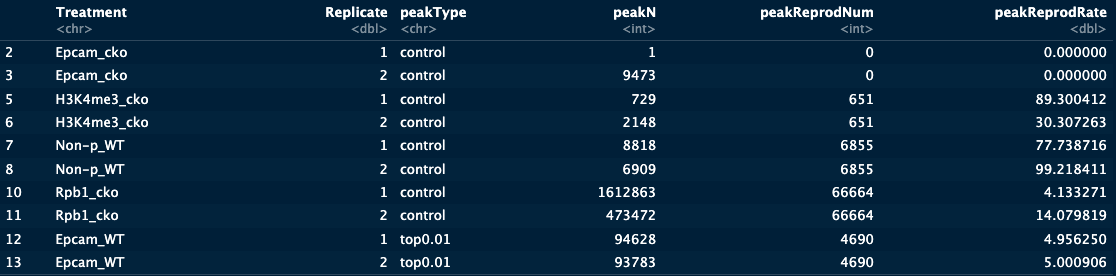
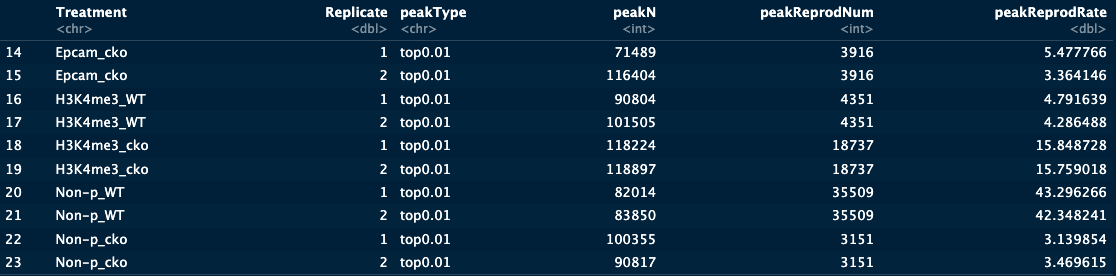

Some samples have no replicated peaks between replicates (peakReprodRate = 0%)
The analysis records adjustments for peakReprodRate > 100 and for samples without replicates. These cases need separate interpretation from the ordinary replicated-peak percentage.
FRagment proportion in Peaks regions (FRiPs)
We calculate the fraction of reads in peaks (FRiPs) as a measure of signal-to-noise and contrast it to FRiPs in the IgG control dataset for illustration. Although sequencing depths for CUT&Tag are typically only 1-5 million reads, the low background of the method results in high FRiP scores.
bamDir = paste0(projPath, "/aligned/sorted/")
inPeakData = c()


## overlap with bam file to get count
  for (sample in Sample) {
    for (rep in c(1,2)) {
      file_path = paste0(projPath, "/peakcalling/seacr/", sample, "_", rep, "_hg38_treat_control.stringent.sort.bed")

      # Check if the file exists and has a non-zero size before reading
      if (file.exists(file_path) && file.info(file_path)$size > 0) {

    peakRes = read.table(file_path, header = FALSE, fill = TRUE)
    peak.gr = GRanges(seqnames = peakRes$V1, IRanges(start = peakRes$V2, end = peakRes$V3), strand = "*")
    bamFile = paste0(bamDir, sample, "_", rep, "_hg38.bam")
    fragment_counts <- getCounts(bamFile, peak.gr, paired = TRUE, by_rg = FALSE, format = "bam")
    inPeakN = counts(fragment_counts)[,1] %>% sum
    inPeakData = rbind(inPeakData, data.frame(inPeakN = inPeakN, Treatment = sample, Replicate = rep))
                        } else {
    print(paste0("The file ", file_path, " contains no peaks"))
                               }
  }
}

inPeakData$Replicate <- factor(inPeakData$Replicate, levels = c(1,2))
frip = left_join(inPeakData, alignResult, by = c("Treatment", "Replicate")) %>%
  mutate(frip = inPeakN/MappedFragNum_hg38 * 100)

frip %>% select(Treatment, Replicate, SequencingDepth, MappedFragNum_hg38, AlignmentRate_hg38, FragInPeakNum = inPeakN, FRiPs = frip)
[1] "The file ~/Shared/CUTandRUN_Wu_Kao_20230828/01_trimmed_reads/results/peakcalling/seacr/Epcam_WT_1_hg38.normalized_20m_treat_control.stringent.sort.bed does not exist or contains no peaks"
Reading in file: ~/Shared/CUTandRUN_Wu_Kao_20230828/01_trimmed_reads/results/aligned/sorted/Epcam_WT_2_hg38.bam
Reading in file: ~/Shared/CUTandRUN_Wu_Kao_20230828/01_trimmed_reads/results/aligned/sorted/Epcam_cko_1_hg38.bam
Reading in file: ~/Shared/CUTandRUN_Wu_Kao_20230828/01_trimmed_reads/results/aligned/sorted/Epcam_cko_2_hg38.bam
Reading in file: ~/Shared/CUTandRUN_Wu_Kao_20230828/01_trimmed_reads/results/aligned/sorted/H3K4me3_WT_1_hg38.bam
[1] "The file ~/Shared/CUTandRUN_Wu_Kao_20230828/01_trimmed_reads/results/peakcalling/seacr/H3K4me3_WT_2_hg38.normalized_20m_treat_control.stringent.sort.bed does not exist or contains no peaks"
Reading in file: ~/Shared/CUTandRUN_Wu_Kao_20230828/01_trimmed_reads/results/aligned/sorted/H3K4me3_cko_1_hg38.bam
Reading in file: ~/Shared/CUTandRUN_Wu_Kao_20230828/01_trimmed_reads/results/aligned/sorted/H3K4me3_cko_2_hg38.bam
Reading in file: ~/Shared/CUTandRUN_Wu_Kao_20230828/01_trimmed_reads/results/aligned/sorted/Non-p_WT_1_hg38.bam
Reading in file: ~/Shared/CUTandRUN_Wu_Kao_20230828/01_trimmed_reads/results/aligned/sorted/Non-p_WT_2_hg38.bam
[1] "The file ~/Shared/CUTandRUN_Wu_Kao_20230828/01_trimmed_reads/results/peakcalling/seacr/Non-p_cko_1_hg38.normalized_20m_treat_control.stringent.sort.bed does not exist or contains no peaks"
[1] "The file ~/Shared/CUTandRUN_Wu_Kao_20230828/01_trimmed_reads/results/peakcalling/seacr/Non-p_cko_2_hg38.normalized_20m_treat_control.stringent.sort.bed does not exist or contains no peaks"
Reading in file: ~/Shared/CUTandRUN_Wu_Kao_20230828/01_trimmed_reads/results/aligned/sorted/Rpb1_WT_1_hg38.bam
[1] "The file ~/Shared/CUTandRUN_Wu_Kao_20230828/01_trimmed_reads/results/peakcalling/seacr/Rpb1_WT_2_hg38.normalized_20m_treat_control.stringent.sort.bed does not exist or contains no peaks"
Reading in file: ~/Shared/CUTandRUN_Wu_Kao_20230828/01_trimmed_reads/results/aligned/sorted/Rpb1_cko_1_hg38.bam
Reading in file: ~/Shared/CUTandRUN_Wu_Kao_20230828/01_trimmed_reads/results/aligned/sorted/Rpb1_cko_2_hg38.bam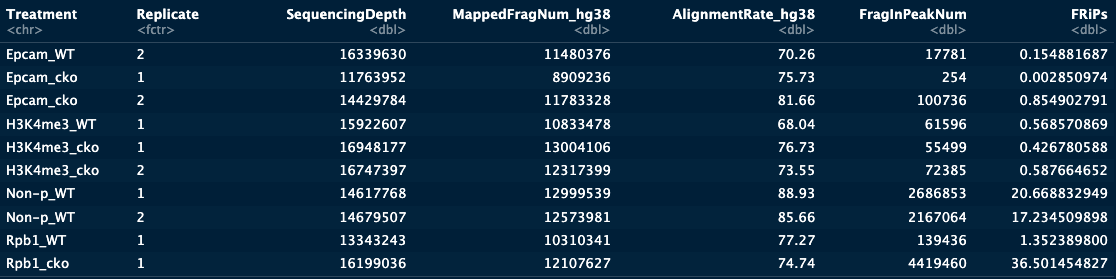

Visualization of peak number, peak width, peak reproducibility and FRiPs
fig7A = peakN %>% ggplot(aes(x = Treatment, y = peakN, fill = Treatment)) +
    geom_boxplot() +
    geom_jitter(aes(color = Replicate), position = position_jitter(0.15)) +
    facet_grid(~peakType) +
    scale_fill_viridis(discrete = TRUE, begin = 0.1, end = 0.55, option = "magma", alpha = 0.8) +
    scale_color_viridis(discrete = TRUE, begin = 0.1, end = 0.9) +
    theme_bw(base_size = 18) +
    ylab("Number of Peaks") +
    xlab("")+
          theme(axis.text.x = element_text(angle = 45,vjust = 1, hjust=1))


fig7B = peakWidth %>% ggplot(aes(x = Treatment, y = width, fill = Treatment)) +
    geom_violin() +
    facet_grid(Replicate~peakType) +
    scale_fill_viridis(discrete = TRUE, begin = 0.1, end = 0.55, option = "magma", alpha = 0.8) +
    scale_color_viridis(discrete = TRUE, begin = 0.1, end = 0.9) +
    scale_y_continuous(trans = "log", breaks = c(400, 3000, 22000)) +
    theme_bw(base_size = 18) +
    ylab("Width of Peaks") +
    xlab("")+
          theme(axis.text.x = element_text(angle = 45,vjust = 1, hjust=1))


fig7C = peakReprod %>% ggplot(aes(x = Treatment, y = peakReprodRate, fill = Treatment, label = round(peakReprodRate, 2))) +
    geom_bar(stat = "identity") +
    geom_text(vjust = 0.1) +
    facet_grid(Replicate~peakType) +
    scale_fill_viridis(discrete = TRUE, begin = 0.1, end = 0.55, option = "magma", alpha = 0.8) +
    scale_color_viridis(discrete = TRUE, begin = 0.1, end = 0.9) +
    theme_bw(base_size = 18) +
    ylab("% of Peaks Reproduced") +
    xlab("")+
          theme(axis.text.x = element_text(angle = 45,vjust = 1, hjust=1))


frip$Replicate = factor(frip$Replicate)
fig7D = frip %>% ggplot(aes(x = Treatment, y = frip, fill = Treatment, label = round(frip, 2))) +
    geom_boxplot() +
    geom_jitter(aes(color = Replicate), position = position_jitter(0.15)) +
    scale_fill_viridis(discrete = TRUE, begin = 0.1, end = 0.55, option = "magma", alpha = 0.8) +
    scale_color_viridis(discrete = TRUE, begin = 0.1, end = 0.9) +
    theme_bw(base_size = 18) +
    ylab("% of Fragments in Peaks (top0.01)") +
    xlab("")+
            theme(axis.text.x = element_text(angle = 45,vjust = 1, hjust=1))


ggarrange(fig7A, fig7B, fig7C, fig7D, ncol = 2, nrow=2, common.legend = TRUE, legend="bottom")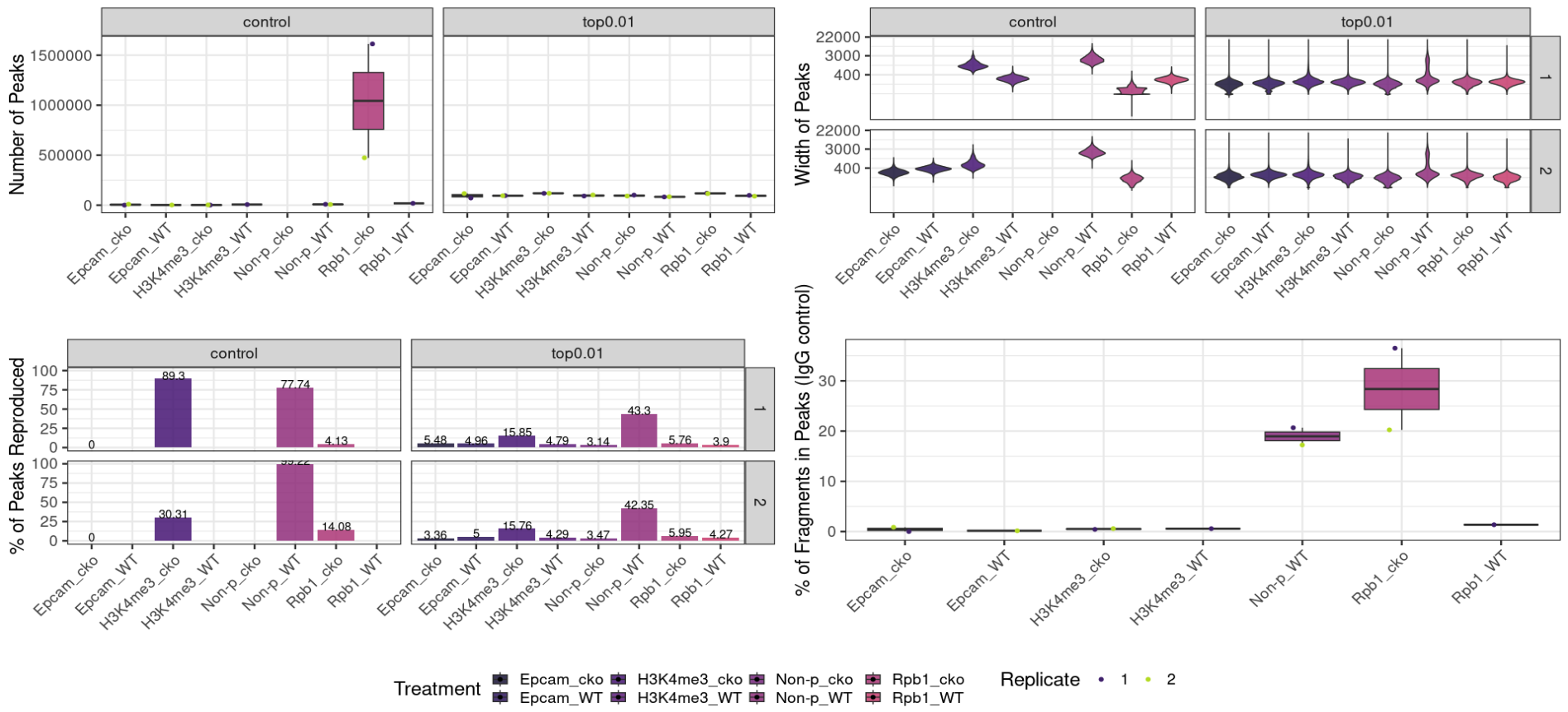
Unfinished analysis: transcription start-site heatmaps
11. Heatmap: TSS
Generating the normalized signal file with BigWig format… (No spike in) and Plot heatmap
bamCoverage
usage: An example usage is:$ bamCoverage -b reads.bam -o coverage.bw

This tool takes an alignment of reads or fragments as input (BAM file) and generates a coverage track (bigWig or bedGraph) as output. The coverage is calculated as the number of reads per bin, where bins are short consecutive counting windows
of a defined size. It is possible to extended the length of the reads to better reflect the actual fragment length. *bamCoverage* offers normalization by scaling factor, Reads Per Kilobase per Million mapped reads (RPKM), counts per million
(CPM), bins per million mapped reads (BPM) and 1x depth (reads per genome coverage, RPGC).

Required arguments:
  --bam BAM file, -b BAM file
                        BAM file to process (default: None)

Output:
  --outFileName FILENAME, -o FILENAME
                        Output file name. (default: None)
  --outFileFormat {bigwig,bedgraph}, -of {bigwig,bedgraph}
                        Output file type. Either "bigwig" or "bedgraph". (default: bigwig)

Optional arguments:
  --help, -h            show this help message and exit
  --scaleFactor SCALEFACTOR
                        The computed scaling factor (or 1, if not applicable) will be multiplied by this. (Default: 1.0)
  --MNase               Determine nucleosome positions from MNase-seq data. Only 3 nucleotides at the center of each fragment are counted. The fragment ends are defined by the two mate reads. Only fragment lengthsbetween 130 - 200 bp are
                        considered to avoid dinucleosomes or other artifacts. By default, any fragments smaller or larger than this are ignored. To over-ride this, use the --minFragmentLength and --maxFragmentLength options, which will
                        default to 130 and 200 if not otherwise specified in the presence of --MNase. *NOTE*: Requires paired-end data. A bin size of 1 is recommended. (default: False)
  --Offset INT [INT ...]
                        Uses this offset inside of each read as the signal. This is useful in cases like RiboSeq or GROseq, where the signal is 12, 15 or 0 bases past the start of the read. This can be paired with the --filterRNAstrand
                        option. Note that negative values indicate offsets from the end of each read. A value of 1 indicates the first base of the alignment (taking alignment orientation into account). Likewise, a value of -1 is the last base
                        of the alignment. An offset of 0 is not permitted. If two values are specified, then they will be used to specify a range of positions. Note that specifying something like --Offset 5 -1 will result in the 5th through
                        last position being used, which is equivalent to trimming 4 bases from the 5-prime end of alignments. Note that if you specify --centerReads, the centering will be performed before the offset. (default: None)
  --filterRNAstrand {forward,reverse}
                        Selects RNA-seq reads (single-end or paired-end) originating from genes on the given strand. This option assumes a standard dUTP-based library preparation (that is, --filterRNAstrand=forward keeps minus-strand reads,
                        which originally came from genes on the forward strand using a dUTP-based method). Consider using --samExcludeFlag instead for filtering by strand in other contexts. (default: None)
  --version             show program's version number and exit
  --binSize INT bp, -bs INT bp
                        Size of the bins, in bases, for the output of the bigwig/bedgraph file. (Default: 50)
  --region CHR:START:END, -r CHR:START:END
                        Region of the genome to limit the operation to - this is useful when testing parameters to reduce the computing time. The format is chr:start:end, for example --region chr10 or --region chr10:456700:891000. (default:
                        None)
  --blackListFileName BED file [BED file ...], -bl BED file [BED file ...]
                        A BED or GTF file containing regions that should be excluded from all analyses. Currently this works by rejecting genomic chunks that happen to overlap an entry. Consequently, for BAM files, if a read partially
                        overlaps a blacklisted region or a fragment spans over it, then the read/fragment might still be considered. Please note that you should adjust the effective genome size, if relevant. (default: None)
  --numberOfProcessors INT, -p INT
                        Number of processors to use. Type "max/2" to use half the maximum number of processors or "max" to use all available processors. (Default: 1)
  --verbose, -v         Set to see processing messages. (default: False)

Read coverage normalization options:
  --effectiveGenomeSize EFFECTIVEGENOMESIZE
                        The effective genome size is the portion of the genome that is mappable. Large fractions of the genome are stretches of NNNN that should be discarded. Also, if repetitive regions were not included in the mapping of
                        reads, the effective genome size needs to be adjusted accordingly. A table of values is available here: http://deeptools.readthedocs.io/en/latest/content/feature/effectiveGenomeSize.html . (default: None)
  --normalizeUsing {RPKM,CPM,BPM,RPGC,None}
                        Use one of the entered methods to normalize the number of reads per bin. By default, no normalization is performed. RPKM = Reads Per Kilobase per Million mapped reads; CPM = Counts Per Million mapped reads, same as CPM
                        in RNA-seq; BPM = Bins Per Million mapped reads, same as TPM in RNA-seq; RPGC = reads per genomic content (1x normalization); Mapped reads are considered after blacklist filtering (if applied). RPKM (per bin) = number
                        of reads per bin / (number of mapped reads (in millions) * bin length (kb)). CPM (per bin) = number of reads per bin / number of mapped reads (in millions). BPM (per bin) = number of reads per bin / sum of all reads
                        per bin (in millions). RPGC (per bin) = number of reads per bin / scaling factor for 1x average coverage. None = the default and equivalent to not setting this option at all. This scaling factor, in turn, is determined
                        from the sequencing depth: (total number of mapped reads * fragment length) / effective genome size. The scaling factor used is the inverse of the sequencing depth computed for the sample to match the 1x coverage. This
                        option requires --effectiveGenomeSize. Each read is considered independently, if you want to only count one mate from a pair in paired-end data, then use the --samFlagInclude/--samFlagExclude options. (Default: None)
  --exactScaling        Instead of computing scaling factors based on a sampling of the reads, process all of the reads to determine the exact number that will be used in the output. This requires significantly more time to compute, but will
                        produce more accurate scaling factors in cases where alignments that are being filtered are rare and lumped together. In other words, this is only needed when region-based sampling is expected to produce incorrect
                        results. (default: False)
  --ignoreForNormalization IGNOREFORNORMALIZATION [IGNOREFORNORMALIZATION ...], -ignore IGNOREFORNORMALIZATION [IGNOREFORNORMALIZATION ...]
                        A list of space-delimited chromosome names containing those chromosomes that should be excluded for computing the normalization. This is useful when considering samples with unequal coverage across chromosomes, like
                        male samples. An usage examples is --ignoreForNormalization chrX chrM. (default: None)
  --skipNonCoveredRegions, --skipNAs
                        This parameter determines if non-covered regions (regions without overlapping reads) in a BAM file should be skipped. The default is to treat those regions as having a value of zero. The decision to skip non-covered
                        regions depends on the interpretation of the data. Non-covered regions may represent, for example, repetitive regions that should be skipped. (default: False)
  --smoothLength INT bp
                        The smooth length defines a window, larger than the binSize, to average the number of reads. For example, if the --binSize is set to 20 and the --smoothLength is set to 60, then, for each bin, the average of the bin
                        and its left and right neighbors is considered. Any value smaller than --binSize will be ignored and no smoothing will be applied. (default: None)

Read processing options:
  --extendReads [INT bp], -e [INT bp]
                        This parameter allows the extension of reads to fragment size. If set, each read is extended, without exception. *NOTE*: This feature is generally NOT recommended for spliced-read data, such as RNA-seq, as it would
                        extend reads over skipped regions. *Single-end*: Requires a user specified value for the final fragment length. Reads that already exceed this fragment length will not be extended. *Paired-end*: Reads with mates are
                        always extended to match the fragment size defined by the two read mates. Unmated reads, mate reads that map too far apart (>4x fragment length) or even map to different chromosomes are treated like single-end reads.
                        The input of a fragment length value is optional. If no value is specified, it is estimated from the data (mean of the fragment size of all mate reads). (default: False)
  --ignoreDuplicates    If set, reads that have the same orientation and start position will be considered only once. If reads are paired, the mate's position also has to coincide to ignore a read. (default: False)
  --minMappingQuality INT
                        If set, only reads that have a mapping quality score of at least this are considered. (default: None)
  --centerReads         By adding this option, reads are centered with respect to the fragment length. For paired-end data, the read is centered at the fragment length defined by the two ends of the fragment. For single-end data, the given
                        fragment length is used. This option is useful to get a sharper signal around enriched regions. (default: False)
  --samFlagInclude INT  Include reads based on the SAM flag. For example, to get only reads that are the first mate, use a flag of 64. This is useful to count properly paired reads only once, as otherwise the second mate will be also
                        considered for the coverage. (Default: None)
  --samFlagExclude INT  Exclude reads based on the SAM flag. For example, to get only reads that map to the forward strand, use --samFlagExclude 16, where 16 is the SAM flag for reads that map to the reverse strand. (Default: None)
  --minFragmentLength INT
                        The minimum fragment length needed for read/pair inclusion. This option is primarily useful in ATACseq experiments, for filtering mono- or di-nucleosome fragments. (Default: 0)
  --maxFragmentLength INT
                        The maximum fragment length needed for read/pair inclusion. (Default: 0)
(bamCoverage in conda is not working, so I use /usr/local/anaconda3/bin/bamCoverage)
mkdir results/aligned/sorted/Heatmap


for ((i = 0; i < ${#samples_cko1[@]}; i+=3)); do
sample_name="${samples[i+2]}"
bam_file=results/aligned/sorted/"$sample_name"_hg38.bam

/usr/local/anaconda3/bin/bamCoverage --bam $bam_file -o results/aligned/sorted/Heatmap/"$sample_name".cpm.norm.bw \
--binSize 30 --normalizeUsing CPM --effectiveGenomeSize 2913022398 \
--numberOfProcessors 80 2> results/log/"$sample_name".gene.bw

done
Create a BED file for the regions of interest (hg38).
awk '$3=="transcript"{OFS="\t";print$1,$4,$5}' Homo_sapiens.GRCh38.104.chr.gtf | sort-bed - | bedtools merge > hg38_transcript.bedcomputeMatrix reference-point
usage: An example usage is:
  computeMatrix reference-point -S <biwig file(s)> -R <bed file> -a 3000 -b 3000

optional arguments:
  -h, --help            show this help message and exit

Required arguments:
  --regionsFileName File [File ...], -R File [File ...]
                        File name or names, in BED or GTF format, containing the regions to plot. If multiple bed files are given, each one is considered a group that can be plotted separately. Also, adding a "#" symbol in the bed file causes
                        all the regions until the previous "#" to be considered one group. (default: None)
  --scoreFileName File [File ...], -S File [File ...]
                        bigWig file(s) containing the scores to be plotted. Multiple files should be separated by spaced. BigWig files can be obtained by using the bamCoverage or bamCompare tools. More information about the bigWig file format
                        can be found at http://genome.ucsc.edu/goldenPath/help/bigWig.html (default: None)

Output options:
  --outFileName OUTFILENAME, -out OUTFILENAME, -o OUTFILENAME
                        File name to save the gzipped matrix file needed by the "plotHeatmap" and "plotProfile" tools. (default: None)
  --outFileNameMatrix FILE
                        If this option is given, then the matrix of values underlying the heatmap will be saved using the indicated name, e.g. IndividualValues.tab.This matrix can easily be loaded into R or other programs. (default: None)
  --outFileSortedRegions BED file
                        File name in which the regions are saved after skiping zeros or min/max threshold values. The order of the regions in the file follows the sorting order selected. This is useful, for example, to generate other heatmaps
                        keeping the sorting of the first heatmap. Example: Heatmap1sortedRegions.bed (default: None)

Optional arguments:
  --version             show program's version number and exit
  --referencePoint {TSS,TES,center}
                        The reference point for the plotting could be either the region start (TSS), the region end (TES) or the center of the region. Note that regardless of what you specify, plotHeatmap/plotProfile will default to using
                        "TSS" as the label. (Default: TSS)
  --beforeRegionStartLength INT bp, -b INT bp, --upstream INT bp
                        Distance upstream of the reference-point selected. (Default: 500)
  --afterRegionStartLength INT bp, -a INT bp, --downstream INT bp
                        Distance downstream of the reference-point selected. (Default: 1500)
  --nanAfterEnd         If set, any values after the region end are discarded. This is useful to visualize the region end when not using the scale-regions mode and when the reference-point is set to the TSS. (default: False)
  --binSize BINSIZE, -bs BINSIZE
                        Length, in bases, of the non-overlapping bins for averaging the score over the regions length. (Default: 10)
  --sortRegions {descend,ascend,no,keep}
                        Whether the output file should present the regions sorted. The default is to not sort the regions. Note that this is only useful if you plan to plot the results yourself and not, for example, with plotHeatmap, which
                        will override this. Note also that unsorted output will be in whatever order the regions happen to be processed in and not match the order in the input files. If you require the output order to match that of the input
                        regions, then either specify "keep" or use computeMatrixOperations to resort the results file. (Default: keep)
  --sortUsing {mean,median,max,min,sum,region_length}
                        Indicate which method should be used for sorting. The value is computed for each row.Note that the region_length option will lead to a dotted line within the heatmap that indicates the end of the regions. (Default:
                        mean)
  --sortUsingSamples SORTUSINGSAMPLES [SORTUSINGSAMPLES ...]
                        List of sample numbers (order as in matrix), that are used for sorting by --sortUsing, no value uses all samples, example: --sortUsingSamples 1 3 (default: None)
  --averageTypeBins {mean,median,min,max,std,sum}
                        Define the type of statistic that should be used over the bin size range. The options are: "mean", "median", "min", "max", "sum" and "std". The default is "mean". (Default: mean)
  --missingDataAsZero   If set, missing data (NAs) will be treated as zeros. The default is to ignore such cases, which will be depicted as black areas in a heatmap. (see the --missingDataColor argument of the plotHeatmap command for
                        additional options). (default: False)
  --skipZeros           Whether regions with only scores of zero should be included or not. Default is to include them. (default: False)
  --minThreshold MINTHRESHOLD
                        Numeric value. Any region containing a value that is less than or equal to this will be skipped. This is useful to skip, for example, genes where the read count is zero for any of the bins. This could be the result of
                        unmappable areas and can bias the overall results. (Default: None)
  --maxThreshold MAXTHRESHOLD
                        Numeric value. Any region containing a value greater than or equal to this will be skipped. The maxThreshold is useful to skip those few regions with very high read counts (e.g. micro satellites) that may bias the
                        average values. (Default: None)
  --blackListFileName BED file, -bl BED file
                        A BED file containing regions that should be excluded from all analyses. Currently this works by rejecting genomic chunks that happen to overlap an entry. Consequently, for BAM files, if a read partially overlaps a
                        blacklisted region or a fragment spans over it, then the read/fragment might still be considered. (default: None)
  --samplesLabel SAMPLESLABEL [SAMPLESLABEL ...]
                        Labels for the samples. This will then be passed to plotHeatmap and plotProfile. The default is to use the file name of the sample. The sample labels should be separated by spaces and quoted if a label itselfcontains a
                        space E.g. --samplesLabel label-1 "label 2" (default: None)
  --smartLabels         Instead of manually specifying labels for the input bigWig and BED/GTF files, this causes deepTools to use the file name after removing the path and extension. (default: False)
  --quiet, -q           Set to remove any warning or processing messages. (default: False)
  --verbose             Being VERY verbose in the status messages. --quiet will disable this. (default: False)
  --scale SCALE         If set, all values are multiplied by this number. (Default: 1)
  --numberOfProcessors INT, -p INT
                        Number of processors to use. Type "max/2" to use half the maximum number of processors or "max" to use all available processors. (Default: 1)

GTF/BED12 options:
  --metagene            When either a BED12 or GTF file are used to provide regions, perform the computation on the merged exons, rather than using the genomic interval defined by the 5-prime and 3-prime most transcript bound (i.e., columns 2
                        and 3 of a BED file). If a BED3 or BED6 file is used as input, then columns 2 and 3 are used as an exon. (Default: False)
  --transcriptID TRANSCRIPTID
                        When a GTF file is used to provide regions, only entries with this value as their feature (column 3) will be processed as transcripts. (Default: transcript)
  --exonID EXONID       When a GTF file is used to provide regions, only entries with this value as their feature (column 3) will be processed as exons. CDS would be another common value for this. (Default: exon)
  --transcript_id_designator TRANSCRIPT_ID_DESIGNATOR
                        Each region has an ID (e.g., ACTB) assigned to it, which for BED files is either column 4 (if it exists) or the interval bounds. For GTF files this is instead stored in the last column as a key:value pair (e.g., as
                        'transcript_id "ACTB"', for a key of transcript_id and a value of ACTB). In some cases it can be convenient to use a different identifier. To do so, set this to the desired key. (Default: transcript_id)

deepBlue arguments:
  Options used only for remote bedgraph/wig files hosted on deepBlue

  --deepBlueURL DEEPBLUEURL
                        For remote files bedgraph/wiggle files hosted on deepBlue, this specifies the server URL. The default is "http://deepblue.mpi-inf.mpg.de/xmlrpc", which should not be changed without good reason. (default:
                        http://deepblue.mpi-inf.mpg.de/xmlrpc)
  --userKey USERKEY     For remote files bedgraph/wiggle files hosted on deepBlue, this specifies the user key to use for access. The default is "anonymous_key", which suffices for public datasets. If you need access to a restricted
                        access/private dataset, then request a key from deepBlue and specify it here. (default: anonymous_key)
  --deepBlueTempDir DEEPBLUETEMPDIR
                        If specified, temporary files from preloading datasets from deepBlue will be written here (note, this directory must exist). If not specified, where ever temporary files would normally be written on your system is
                        used. (default: None)
  --deepBlueKeepTemp    If specified, temporary bigWig files from preloading deepBlue datasets are not deleted. A message will be printed noting where these files are and what sample they correspond to. These can then be used if you wish to
                        analyse the same sample with the same regions again. (default: False)
for ((i = 0; i < ${#samples_cko1[@]}; i+=3)); do
sample_name="${samples[i+2]}"
/usr/local/anaconda3/bin/computeMatrix reference-point \
--referencePoint TSS -b 3000 -a 3000 \
-R hg38_transcript.bed \
-S results/aligned/sorted/Heatmap/"$sample_name".cpm.norm.bw --skipZeros \
--outFileName results/aligned/sorted/Heatmap/matrix1_"$sample_name"_TSS.gz
doneplotHeatmap
usage: plotHeatmap [--matrixFile MATRIXFILE] --outFileName OUTFILENAME [--outFileSortedRegions FILE] [--outFileNameMatrix FILE] [--interpolationMethod STR] [--dpi DPI] [--kmeans KMEANS] [--hclust HCLUST] [--silhouette] [--help] [--version]
                   [--plotType {lines,fill,se,std}] [--sortRegions {descend,ascend,no,keep}] [--sortUsing {mean,median,max,min,sum,region_length}] [--sortUsingSamples SORTUSINGSAMPLES [SORTUSINGSAMPLES ...]] [--linesAtTickMarks]
                   [--clusterUsingSamples CLUSTERUSINGSAMPLES [CLUSTERUSINGSAMPLES ...]] [--averageTypeSummaryPlot {mean,median,min,max,std,sum}] [--missingDataColor MISSINGDATACOLOR] [--colorMap COLORMAP [COLORMAP ...]] [--alpha ALPHA]
                   [--colorList COLORLIST [COLORLIST ...]] [--colorNumber COLORNUMBER] [--zMin ZMIN [ZMIN ...]] [--zMax ZMAX [ZMAX ...]] [--heatmapHeight HEATMAPHEIGHT] [--heatmapWidth HEATMAPWIDTH]
                   [--whatToShow {plot, heatmap and colorbar,plot and heatmap,heatmap only,heatmap and colorbar}] [--boxAroundHeatmaps BOXAROUNDHEATMAPS] [--xAxisLabel XAXISLABEL] [--startLabel STARTLABEL] [--endLabel ENDLABEL]
                   [--refPointLabel REFPOINTLABEL] [--labelRotation LABEL_ROTATION] [--regionsLabel REGIONSLABEL [REGIONSLABEL ...]] [--samplesLabel SAMPLESLABEL [SAMPLESLABEL ...]] [--plotTitle PLOTTITLE] [--yAxisLabel YAXISLABEL]
                   [--yMin YMIN [YMIN ...]] [--yMax YMAX [YMAX ...]] [--legendLocation {best,upper-right,upper-left,upper-center,lower-left,lower-right,lower-center,center,center-left,center-right,none}] [--perGroup] [--plotFileFormat]
                   [--verbose]

This tool creates a heatmap for scores associated with genomic regions. The program requires a matrix file generated by the tool ``computeMatrix``.

Required arguments:
  --matrixFile MATRIXFILE, -m MATRIXFILE
                        Matrix file from the computeMatrix tool. (default: None)
  --outFileName OUTFILENAME, -out OUTFILENAME, -o OUTFILENAME
                        File name to save the image to. The file ending will be used to determine the image format. The available options are: "png", "eps", "pdf" and "svg", e.g., MyHeatmap.png. (default: None)

Output options:
  --outFileSortedRegions FILE
                        File name into which the regions are saved after skipping zeros or min/max threshold values. The order of the regions in the file follows the sorting order selected. This is useful, for example, to generate other
                        heatmaps while keeping the sorting of the first heatmap. Example: Heatmap1sortedRegions.bed (default: None)
  --outFileNameMatrix FILE
                        If this option is given, then the matrix of values underlying the heatmap will be saved using this name, e.g. MyMatrix.gz. (default: None)
  --interpolationMethod STR
                        If the heatmap image contains a large number of columns is usually better to use an interpolation method to produce better results (see
                        https://matplotlib.org/examples/images_contours_and_fields/interpolation_methods.html). Be default, plotHeatmap uses the method `nearest` if the number of columns is 1000 or less. Otherwise it uses the bilinear method.
                        This default behaviour can be changed by using any of the following options: "nearest", "bilinear", "bicubic", "gaussian" (default: auto)
  --dpi DPI             Set the DPI to save the figure. (default: 200)

Clustering arguments:
  --kmeans KMEANS       Number of clusters to compute. When this option is set, the matrix is split into clusters using the k-means algorithm. Only works for data that is not grouped, otherwise only the first group will be clustered. If more
                        specific clustering methods are required, then save the underlying matrix and run the clustering using other software. The plotting of the clustering may fail with an error if a cluster has very few members compared to
                        the total number or regions. (default: None)
  --hclust HCLUST       Number of clusters to compute. When this option is set, then the matrix is split into clusters using the hierarchical clustering algorithm, using "ward linkage". Only works for data that is not grouped, otherwise only
                        the first group will be clustered. --hclust could be very slow if you have >1000 regions. In those cases, you might prefer --kmeans or if more clustering methods are required you can save the underlying matrix and run
                        the clustering using other software. The plotting of the clustering may fail with an error if a cluster has very few members compared to the total number of regions. (default: None)
  --silhouette          Compute the silhouette score for regions. This is only applicable if clustering has been performed. The silhouette score is a measure of how similar a region is to other regions in the same cluster as opposed to those
                        in other clusters. It will be reported in the final column of the BED file with regions. The silhouette evaluation can be very slow when you have morethan 100 000 regions. (default: False)

Optional arguments:
  --help, -h            show this help message and exit
  --version             show program's version number and exit
  --plotType {lines,fill,se,std}
                        "lines" will plot the profile line based on the average type selected. "fill" fills the region between zero and the profile curve. The fill in color is semi transparent to distinguish different profiles. "se" and "std"
                        color the region between the profile and the standard error or standard deviation of the data. (default: lines)
  --sortRegions {descend,ascend,no,keep}
                        Whether the heatmap should present the regions sorted. The default is to sort in descending order based on the mean value per region. Note that "keep" and "no" are the same thing. (default: descend)
  --sortUsing {mean,median,max,min,sum,region_length}
                        Indicate which method should be used for sorting. For each row the method is computed. For region_length, a dashed line is drawn at the end of the region (reference point TSS and center) or the beginning of the region
                        (reference point TES) as appropriate. (default: mean)
  --sortUsingSamples SORTUSINGSAMPLES [SORTUSINGSAMPLES ...]
                        List of sample numbers (order as in matrix), which are used by --sortUsing for sorting. If no value is set, it uses all samples. Example: --sortUsingSamples 1 3 (default: None)
  --linesAtTickMarks    Draw dashed lines from all tick marks through the heatmap. This is then similar to the dashed line draw at region bounds when using a reference point and --sortUsing region_length (default: False)
  --clusterUsingSamples CLUSTERUSINGSAMPLES [CLUSTERUSINGSAMPLES ...]
                        List of sample numbers (order as in matrix), that are used for clustering by --kmeans or --hclust if not given, all samples are taken into account for clustering. Example: --ClusterUsingSamples 1 3 (default: None)
  --averageTypeSummaryPlot {mean,median,min,max,std,sum}
                        Define the type of statistic that should be plotted in the summary image above the heatmap. The options are: "mean", "median", "min", "max", "sum" and "std". (default: mean)
  --missingDataColor MISSINGDATACOLOR
                        If --missingDataAsZero was not set, such cases will be colored in black by default. Using this parameter, a different color can be set. A value between 0 and 1 will be used for a gray scale (black is 0). For a list of
                        possible color names see: http://packages.python.org/ete2/reference/reference_svgcolors.html. Other colors can be specified using the #rrggbb notation. (default: black)
  --colorMap COLORMAP [COLORMAP ...]
                        Color map to use for the heatmap. If more than one heatmap is being plotted the color of each heatmap can be enter individually (e.g. `--colorMap Reds Blues`). Color maps are recycled if the number of color maps is
                        smaller than the number of heatmaps being plotted. Available values can be seen here: http://matplotlib.org/users/colormaps.html The available options are: 'magma', 'inferno', 'plasma', 'viridis', 'cividis',
                        'twilight', 'twilight_shifted', 'turbo', 'Blues', 'BrBG', 'BuGn', 'BuPu', 'CMRmap', 'GnBu', 'Greens', 'Greys', 'OrRd', 'Oranges', 'PRGn', 'PiYG', 'PuBu', 'PuBuGn', 'PuOr', 'PuRd', 'Purples', 'RdBu', 'RdGy', 'RdPu',
                        'RdYlBu', 'RdYlGn', 'Reds', 'Spectral', 'Wistia', 'YlGn', 'YlGnBu', 'YlOrBr', 'YlOrRd', 'afmhot', 'autumn', 'binary', 'bone', 'brg', 'bwr', 'cool', 'coolwarm', 'copper', 'cubehelix', 'flag', 'gist_earth', 'gist_gray',
                        'gist_heat', 'gist_ncar', 'gist_rainbow', 'gist_stern', 'gist_yarg', 'gnuplot', 'gnuplot2', 'gray', 'hot', 'hsv', 'jet', 'nipy_spectral', 'ocean', 'pink', 'prism', 'rainbow', 'seismic', 'spring', 'summer', 'terrain',
                        'winter', 'Accent', 'Dark2', 'Paired', 'Pastel1', 'Pastel2', 'Set1', 'Set2', 'Set3', 'tab10', 'tab20', 'tab20b', 'tab20c', 'rocket', 'mako', 'vlag', 'icefire' (default: ['RdYlBu'])
  --alpha ALPHA         The alpha channel (transparency) to use for the heatmaps. The default is 1.0 and values must be between 0 and 1. (default: 1.0)
  --colorList COLORLIST [COLORLIST ...]
                        List of colors to use to create a colormap. For example, if `--colorList black,yellow,blue` is set (colors separated by comas) then a color map that starts with black, continues to yellow and finishes in blue is
                        created. If this option is selected, it overrides the --colorMap chosen. The list of valid color names can be seen here: http://matplotlib.org/examples/color/named_colors.html Hex colors are valid (e.g #34a2b1). If
                        individual colors for different heatmaps need to be specified they need to be separated by space as for example: `--colorList "white,#cccccc" "white,darkred"` As for --colorMap, the color lists are recycled if their
                        number is smaller thatn the number ofplotted heatmaps. The number of transitions is defined by the --colorNumber option. (default: None)
  --colorNumber COLORNUMBER
                        N.B., --colorList is required for an effect. This controls the number of transitions from one color to the other. If --colorNumber is the number of colors in --colorList then there will be no transitions between the
                        colors. (default: 256)
  --zMin ZMIN [ZMIN ...], -min ZMIN [ZMIN ...]
                        Minimum value for the heatmap intensities. Multiple values, separated by spaces can be set for each heatmap. If the number of zMin values is smaller thanthe number of heatmaps the values are recycled. If a value is set
                        to "auto", it will be set to the first percentile of the matrix values. (default: None)
  --zMax ZMAX [ZMAX ...], -max ZMAX [ZMAX ...]
                        Maximum value for the heatmap intensities. Multiple values, separated by spaces can be set for each heatmap. If the number of zMax values is smaller thanthe number of heatmaps the values are recycled. If a value is set
                        to "auto", it will be set to the 98th percentile of the matrix values. (default: None)
  --heatmapHeight HEATMAPHEIGHT
                        Plot height in cm. The default for the heatmap height is 28. The minimum value is 3 and the maximum is 100. (default: 28)
  --heatmapWidth HEATMAPWIDTH
                        Plot width in cm. The default value is 4 The minimum value is 1 and the maximum is 100. (default: 4)
  --whatToShow {plot, heatmap and colorbar,plot and heatmap,heatmap only,heatmap and colorbar}
                        The default is to include a summary or profile plot on top of the heatmap and a heatmap colorbar. Other options are: "plot and heatmap", "heatmap only", "heatmap and colorbar", and the default "plot, heatmap and
                        colorbar". (default: plot, heatmap and colorbar)
  --boxAroundHeatmaps BOXAROUNDHEATMAPS
                        By default black boxes are plot around heatmaps. This can be turned off by setting --boxAroundHeatmaps no (default: yes)
  --xAxisLabel XAXISLABEL, -x XAXISLABEL
                        Description for the x-axis label. (default: gene distance (bp))
  --startLabel STARTLABEL
                        [only for scale-regions mode] Label shown in the plot for the start of the region. Default is TSS (transcription start site), but could be changed to anything, e.g. "peak start". Same for the --endLabel option. See
                        below. (default: TSS)
  --endLabel ENDLABEL   [only for scale-regions mode] Label shown in the plot for the region end. Default is TES (transcription end site). (default: TES)
  --refPointLabel REFPOINTLABEL
                        [only for reference-point mode] Label shown in the plot for the reference-point. Default is the same as the reference point selected (e.g. TSS), but could be anything, e.g. "peak start". (default: None)
  --labelRotation LABEL_ROTATION
                        Rotation of the X-axis labels in degrees. The default is 0, positive values denote a counter-clockwise rotation. (default: 0.0)
  --regionsLabel REGIONSLABEL [REGIONSLABEL ...], -z REGIONSLABEL [REGIONSLABEL ...]
                        Labels for the regions plotted in the heatmap. If more than one region is being plotted, a list of labels separated by spaces is required. If a label itself contains a space, then quotes are needed. For example,
                        --regionsLabel label_1, "label 2". (default: None)
  --samplesLabel SAMPLESLABEL [SAMPLESLABEL ...]
                        Labels for the samples plotted. The default is to use the file name of the sample. The sample labels should be separated by spaces and quoted if a label itselfcontains a space E.g. --samplesLabel label-1 "label 2"
                        (default: None)
  --plotTitle PLOTTITLE, -T PLOTTITLE
                        Title of the plot, to be printed on top of the generated image. Leave blank for no title. (default: )
  --yAxisLabel YAXISLABEL, -y YAXISLABEL
                        Y-axis label for the top panel. (default: )
  --yMin YMIN [YMIN ...]
                        Minimum value for the Y-axis. Multiple values, separated by spaces can be set for each profile. If the number of yMin values is smaller thanthe number of plots, the values are recycled. (default: None)
  --yMax YMAX [YMAX ...]
                        Maximum value for the Y-axis. Multiple values, separated by spaces can be set for each profile. If the number of yMin values is smaller thanthe number of plots, the values are recycled. (default: None)
  --legendLocation {best,upper-right,upper-left,upper-center,lower-left,lower-right,lower-center,center,center-left,center-right,none}
                        Location for the legend in the summary plot. Note that "none" does not work for the profiler. (default: best)
  --perGroup            The default is to plot all groups of regions by sample. Using this option instead plots all samples by group of regions. Note that this is only useful if you have multiple groups of regions. by sample rather than
                        group. (default: False)
  --plotFileFormat      Image format type. If given, this option overrides the image format based on the plotFile ending. The available options are: "png", "eps", "pdf", "plotly" and "svg" (default: None)
  --verbose             If set, warning messages and additional information are given. (default: False)

An example usage is: plotHeatmap -m <matrix file>
for ((i = 0; i < ${#samples_cko1[@]}; i+=3)); do
sample_name="${samples[i+2]}"
/usr/local/anaconda3/bin/plotHeatmap -m results/aligned/sorted/Heatmap/matrix1_"$sample_name"_TSS.gz -out Hmp_matrix1_"$sample_name".png