Bulk RNA-seq pairwise comparisons

Goal

Discover the DEGs between WT and KO samples
ORA analysis (OrgDb & MSigDb: C5 group)
GSEA

Example

Samples (experimental design)

WT1 WT2 WT3 KO1 KO2 KO3

1. Discover the DEGs between WT and KO samples

Library and Data Import

library(DESeq2)
library(ashr)
library(sva)    # for batch correction
library(corrplot)    # for correlation plot
library(ggvenn)    # for Venn Diagram
library(car)  # point labels without overlaps
library(umap) # umap
library(tibble)

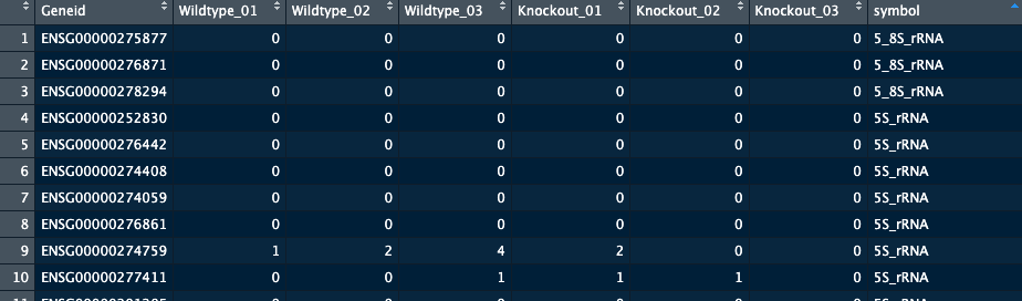
Import raw count matrix and transfer Ensembl ID to Symbol

count_matrix <- read_delim("###", 
                           delim = "\t", 
                           escape_double = FALSE, 
                           trim_ws = TRUE)
symbol <- read_delim("###", 
                     delim = "\t", 
                     escape_double = FALSE, 
                     trim_ws = TRUE)
symbol2 <- symbol[,c(1:2)]
colnames(symbol2) = c("Gene","symbol")


count_matrix <- count_matrix %>% column_to_rownames(var="Geneid")

Different Ensembl IDs can map to the same gene symbol, so I deferred symbol conversion until later in the workflow.

metadata <- read_delim("..///metadata.txt",
                           delim = "\\t",
                           escape_double = FALSE,
                           trim_ws = TRUE)

metadata$group <- factor(metadata$group, levels = c("WT","KO"))
metadata$rep <- factor(metadata$rep, levels = c("1","2","3"))

Pre-filtering

# eliminate rows with NAs
count_matrix <- na.omit(count_matrix)
# no change

# are there duplicated geneID?
length(unique(rownames(count_matrix)))
# no


# the read count cut-off of the low-expression genes
low_exp_read_count = 5
# minimum samples that express this gene (總共有 6 個 sample)
minimum_exp_sample = 2

DEseq2

dds_batch <- DESeqDataSetFromMatrix(countData= round(count_matrix), 
                              colData= metadata, 
                              design= ~rep + group) # 要看是否有 batch effect 來變動 design = ~batch + group



# 至少在 >= 2 個 sample 中有 >5 的表達
keep <- rowSums(counts(dds_batch) > low_exp_read_count) >= minimum_exp_sample
dds_batch <- dds_batch[keep, ] 

# 58884 -> 19903 genes

# Size factor
dds_batch<-estimateSizeFactors(dds_batch)

dds_batch_wald <- DESeq(dds_batch,
              test = "Wald",
              fitType = "parametric",
              betaPrior = F) #  whether or not to put a zero-mean normal prior on the non-intercept coefficients


summary(results(dds_batch_wald))


plotDispEsts(dds_batch_wald)

out of 19903 with nonzero total read count
adjusted p-value < 0.1
LFC > 0 (up)       : 2128, 11%
LFC < 0 (down)     : 2678, 13%
outliers [1]       : 0, 0%
low counts [2]     : 4245, 21%
(mean count < 13)
[1] see 'cooksCutoff' argument of ?results
[2] see 'independentFiltering' argument of ?results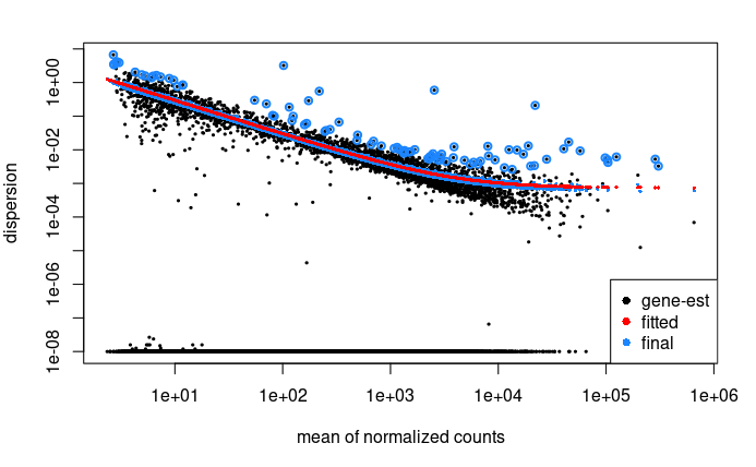

result_KO_WT_batch <-results(dds_batch_wald,
                      contrast=c("group","KO","WT"), # base factor level 放後面
                      alpha = 0.05,
                      lfcThreshold = 0, # default
                      independentFiltering = TRUE,
                      pAdjustMethod = "fdr")

# (genes' logFC > 0 表示 genes are overexpressed in "KO" group)


result_KO_WT_batch_df <- as.data.frame(result_KO_WT_batch)
result_KO_WT_batch_df <- result_KO_WT_batch_df[order(result_KO_WT_batch_df$padj),]

write.csv(result_KO_WT_batch_df, file = "###")

# check if any genes has baseMean = 0?
result_KO_WT_batch_df[result_KO_WT_batch_df$baseMean == 0,]
# 0 genes

# check if there are any outlier( pvalue and padj = NA? )?
result_KO_WT_batch_df[is.na(result_KO_WT_batch_df$pvalue) & is.na(result_KO_WT_batch_df$padj),]
# 0 outliers



# check how many genes were filtered by automatic independent filtering, for having a low mean normalized count: only padj = NA?
result_KO_WT_batch_df[is.na(result_KO_WT_batch_df$padj) & !is.na(result_KO_WT_batch_df$pvalue),]
# -> 有 4631 個 genes 被 independent filtered


metadata(result_KO_WT_batch)$filterThreshold
# DESeq2 has filtered out genes with a mean count of 14.73549
# as a result, 23.26531% of genes were filtered out of the analysis

lfcShrink

# "apeglm"
result_KO_WT_batch_shrink_apeglm <- lfcShrink(dds_batch_wald,
                                         type="apeglm",
                                         coef = "group_KO_vs_WT",
                                         res = result_KO_WT_batch)


# "ashr"
result_KO_WT_batch_shrink_ashr <- lfcShrink(dds_batch_wald,
                                      type="ashr",
                                      res = result_KO_WT_batch)

# normal
result_KO_WT_batch_shrink_normal <- lfcShrink(dds_batch_wald,
                                      type="normal",
                                      coef = "group_KO_vs_WT",
                                      res = result_KO_WT_batch)


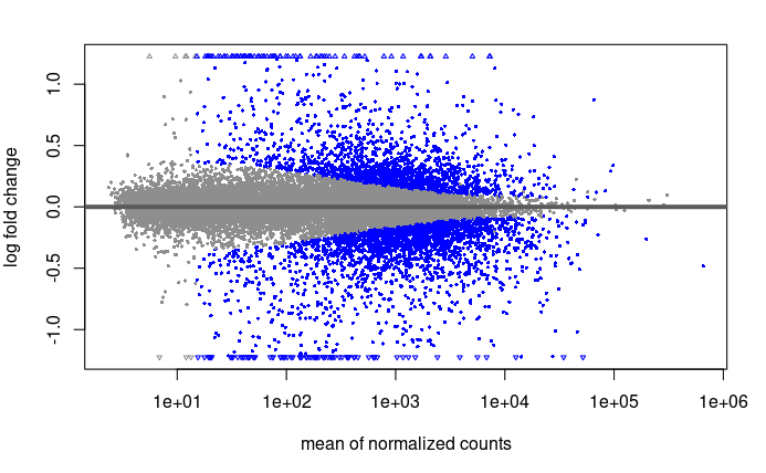
plotMA(result_KO_WT_batch)
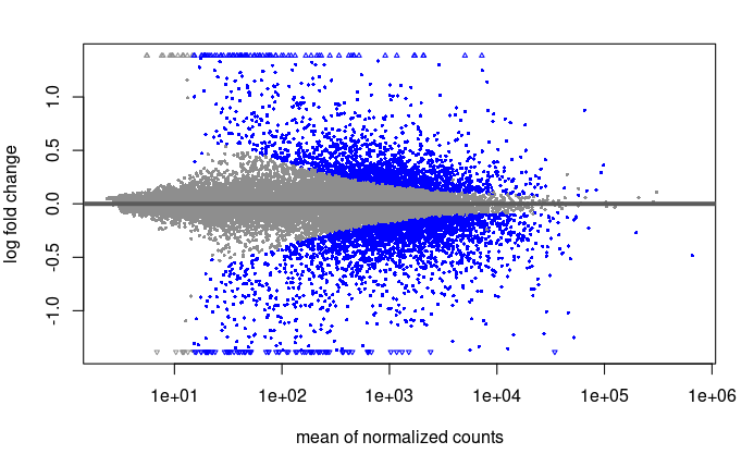
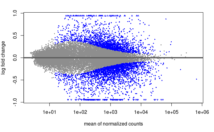
# If you see a lot of variability or small fold changes, "apeglm" might be more appropriate. If there is a trend of variance changing with average expression, "ashr" could be a good choice.

plotMA(result_KO_WT_batch_shrink_ashr)
plotMA(result_KO_WT_batch_shrink_apeglm)
plotMA(result_KO_WT_batch_shrink_normal)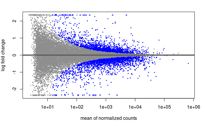

result_KO_WT_batch_shrink_ashr_df <- as.data.frame(result_KO_WT_batch_shrink_ashr)
result_KO_WT_batch_shrink_ashr_df <- result_KO_WT_batch_shrink_ashr_df[order(result_KO_WT_batch_shrink_ashr_df$padj),]


write.csv(result_KO_WT_batch_shrink_ashr_df, file = "###")

Subset DEGs (padj < 0.005)

result_KO_WT_batch_shrink_df_subset.padj2 <- subset(result_KO_WT_batch_shrink_ashr_df, 
                                 (result_KO_WT_batch_shrink_ashr_df$padj < 0.005 & 
                                  abs(result_KO_WT_batch_shrink_ashr_df$log2FoldChange) > 1))


result_KO_WT_batch_shrink_df_subset.padj2 <- tibble::rownames_to_column(result_KO_WT_batch_shrink_df_subset.padj2, "Gene")
# -> 249 DEGs


# concact with normalized counts
result_KO_WT_batch_shrink_df_subset.padj2 <- merge(result_KO_WT_batch_shrink_df_subset.padj2, 
                                            normalized_counts,
                                            by = "Gene")

write.csv(result_KO_WT_batch_shrink_df_subset.padj2, file = "###")

Volcano plot

result_KO_WT_batch_shrink_ashr_df <- result_KO_WT_batch_shrink_ashr_df %>% rownames_to_column("Gene")
result_KO_WT_batch_shrink_ashr_df <- merge(result_KO_WT_batch_shrink_ashr_df, symbol2, by = "Gene")

library(EnhancedVolcano)

# if there are outliers
#res$log2FoldChange_new <- ifelse(abs(res$log2FoldChange) > 6, 6, res$log2FoldChange)
#shape_vector <- ifelse(abs(res$log2FoldChange) > 6, 18, 20)


volcano_plot_batch <- EnhancedVolcano(result_KO_WT_batch_shrink_ashr_df,
                lab = result_KO_WT_batch_shrink_ashr_df$symbol,
                x="log2FoldChange",
                y="padj",
                pCutoff = 0.005,
                FCcutoff = 1,
                labSize = 2,
                legendLabels=c('Not significant',
                               '|Log (base 2) FC| > 1',
                               'p-adj < 0.005',
                               'p-adj & Log (base 2) FC'),
                subtitle = "19903 genes in total",
                title = 'Volcano plot (lfcShrink)',
                #shape = shape_vector,   # if there are outliers
                caption = "") 

pdf(file = "DEG_KO-vs-WT/Batch_correction/volcano_plot.pdf", height = 5, width = 10)
volcano_plot_batch
dev.off()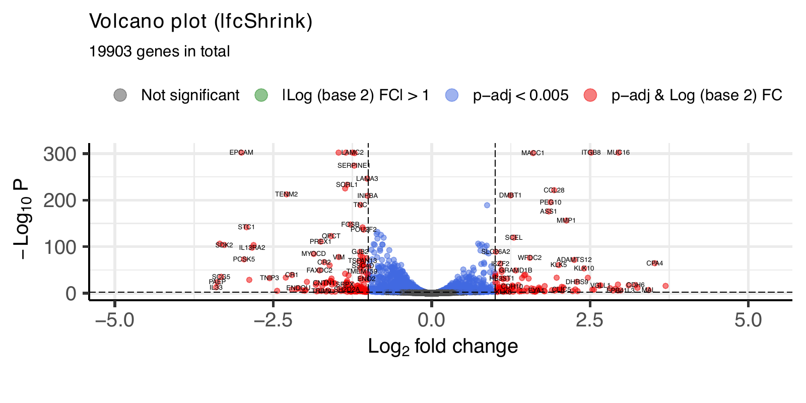

volcano_plot.pdf

DEG heatmap from vst matrix

vst matrix here has to remove the batch effect

vst_batch <- vst(dds_batch, blind=FALSE)

mat <- assay(vst_batch)
mm <- model.matrix(~group, colData(vst_batch))
mat <- limma::removeBatchEffect(mat, batch=vst_batch$rep, design=mm)
assay(vst_batch) <- mat
plotPCA(vst_batch,intgroup="rep")
plotPCA(vst_batch,intgroup="group")




vst_mat_batch <- as.data.frame(assay(vst_batch))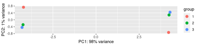

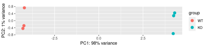
vst matrix here has to remove the batch effect

vst_batch_sig_padj <- vst_mat_batch[rownames(vst_mat_batch) %in% result_KO_WT_batch_shrink_df_subset.padj2$Gene,]

# scale and centering
vst_batch_sig_padj_scale <- t(scale(t(vst_batch_sig_padj))) # scale each genes
vst_batch_sig_padj_scale_df <- as.data.frame(vst_batch_sig_padj_scale)


# set color and break
vst_batch_sig_padj_scale_df[vst_batch_sig_padj_scale_df < -1.5] <- -1.5
vst_batch_sig_padj_scale_df[vst_batch_sig_padj_scale_df > 1.5] <- 1.5

vst_batch_sig_padj_scale_df <- vst_batch_sig_padj_scale_df %>% rownames_to_column("Gene")
vst_batch_sig_padj_scale_df <- merge(vst_batch_sig_padj_scale_df, symbol2, by = "Gene")
vst_batch_sig_padj_scale_df <- vst_batch_sig_padj_scale_df[,-c(1)]





newnames <- lapply(
  vst_batch_sig_padj_scale_df$symbol,
  function(x) bquote(italic(.(x))))


###################################
########### heatmap ###############
###################################
hmap_vst_batch_sig_padj_scale <- pheatmap::pheatmap(vst_batch_sig_padj_scale_df[,-c(7)],
         show_rownames = T,
         breaks=seq(from=-1.5, to=1.5, length=101),
         fontsize_row = 2,
         labels_row = as.expression(newnames),
         cluster_col=FALSE,
         angle_col = "45",
         cluster_rows = TRUE,
         clustering_distance_rows = "euclidean",
         clustering_method = "ward.D2",
         border_color = NA,
         main = "DEG_padj<0.005: vst_counts_scaled\n (scaled for each gene, 249 DEGs in total, \nremove batch effect),\nbreak: 0 \u00b1 1.5, euclidean, ward.D2")


pdf(file = "###",height = 9,width = 5)
hmap_vst_batch_sig_padj_scale
dev.off()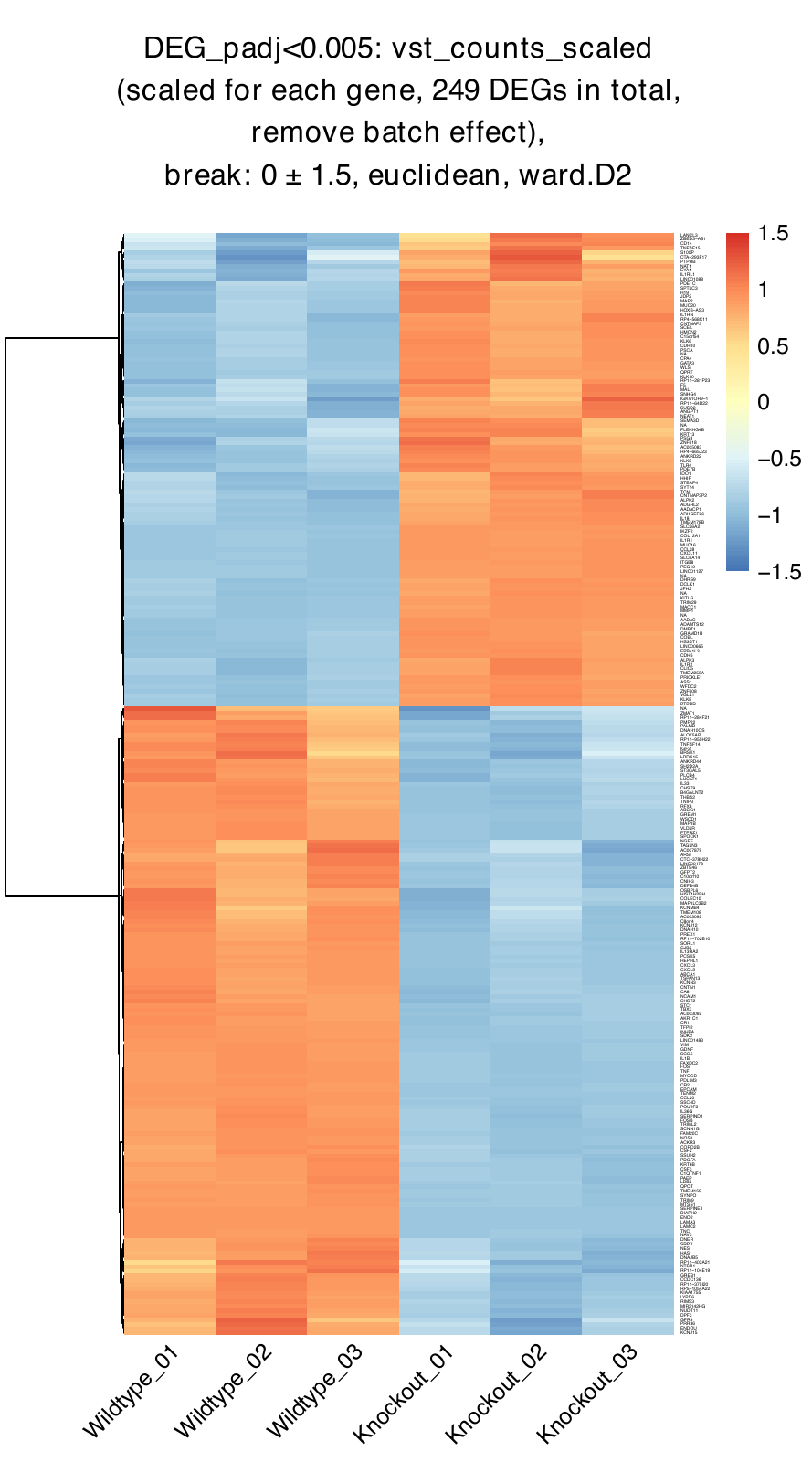

heatmap_DEGs_padj0.005.pdf

2. ORA analysis (OrgDb & MSigDb: C5 group)

Library and Data Import

library(DESeq2)
library(ashr)
library(sva)    # for batch correction
library(corrplot)    # for correlation plot
library(ggvenn)    # for Venn Diagram
library(car)  # point labels without overlaps
library(umap) # umap
library(tibble)
library(clusterProfiler)
library(msigdbr)
library(org.Hs.eg.db)


# import DEG subset results (p<0.005, batch corrected)
DEGs_KOvsWT <- read_csv("###",
                        col_types = cols(...1 = col_skip()))

ORA (OrgDb)

# down regulated: genes are down-expressed in "KO" group)
GO.KOvsWT.down <- enrichGO(gene = DEGs_KOvsWT[DEGs_KOvsWT$log2FoldChange<0,]$Gene,
                           OrgDb = org.Hs.eg.db,
                           keyType = "ENSEMBL",
                           ont = "ALL",
                           pAdjustMethod = "fdr",
                           pvalueCutoff = 0.05,
                           qvalueCutoff = 0.1,
                           minGSSize = 10,
                           maxGSSize = 800,
                           readable = T)

# up regulated: genes are up-expressed in "KO" group)
GO.KOvsWT.up <- enrichGO(gene = DEGs_KOvsWT[DEGs_KOvsWT$log2FoldChange>0,]$Gene,
                                OrgDb = org.Hs.eg.db,
                                keyType = "ENSEMBL",
                                ont = "ALL",
                                pAdjustMethod = "fdr",
                                pvalueCutoff = 0.05,
                                qvalueCutoff = 0.1,
                                minGSSize = 10,
                                maxGSSize = 800,
                                readable = T)



# 根據 gene count 數量來filter GO:
# down regulated genes
GO.KOvsWT.down.filter <- gsfilter(GO.KOvsWT.down, by = "Count", min = 5) # 156 -> 106
GO.KOvsWT.down.filter@result

write.csv(GO.KOvsWT.down.filter@result,
          file="###",
          row.names = FALSE,
          quote = FALSE)

# up regulated genes
GO.KOvsWT.up.filter <- gsfilter(GO.KOvsWT.up, by = "Count", min = 5)
GO.KOvsWT.up.filter@result

write.csv(GO.KOvsWT.up.filter@result,
          file="###",
          row.names = FALSE,
          quote = FALSE)

Visualization

Dotplot

pdf(file = "###")
dotplot(GO.KOvsWT.down.filter,
                         split="ONTOLOGY",
                         showCategory = 8,
                         font.size = 8)+
              facet_grid(ONTOLOGY~.,
                         scale="free")+
              ggtitle("Dotplot of GO of DEGs (down-regulated in KO)")
dev.off()

pdf(file = "###")
dotplot(GO.KOvsWT.up.filter,
                         split="ONTOLOGY",
                         showCategory = 8,
                         font.size = 8)+
              facet_grid(ONTOLOGY~.,
                         scale="free")+
              ggtitle("Dotplot of GO of DEGs (up-regulated in KO)")
dev.off()

Emaplot

GO.KOvsWT.down.filter <-enrichplot::pairwise_termsim(GO.KOvsWT.down.filter)
GO.KOvsWT.up.filter <-enrichplot::pairwise_termsim(GO.KOvsWT.up.filter)


pdf(file = "###")
enrichplot::emapplot(GO.KOvsWT.down.filter,
                     showCategory = 20,
                     cex.params = list(category_label = 0.5,
                                       category_node = 0.5),
                     layout.params = list(layout = "kk"))+
  ggtitle("emapplot of GO of DEGs (down-regulated in KO)")
dev.off()


pdf(file = "###")
enrichplot::emapplot(GO.KOvsWT.up.filter,
                     showCategory = 20,
                     cex.params = list(category_label = 0.5,
                                       category_node = 0.5),
                     layout.params = list(layout = "kk"))+
  ggtitle("emapplot of GO of DEGs (up-regulated in KO)")
dev.off()

ORA (MSigDb: C5 group)

Retrieve interested human gene sets

# C5
MSigDb.human.c5 <- msigdbr(species = "Homo sapiens",
                           category = "C5") %>%
  dplyr::select(gs_name,gs_subcat, ensembl_gene)

MSigDb.human.c5 <- MSigDb.human.c5[MSigDb.human.c5$gs_subcat != "HPO",][,-c(2)]



# C3
MSigDb.human.c3 <- msigdbr(species = "Homo sapiens",
                           category = "C3") %>%
  dplyr::select(gs_name, gs_subcat,ensembl_gene)

MSigDb.human.c3 <- MSigDb.human.c3[MSigDb.human.c3$gs_subcat %in% c("TFT:TFT_Legacy",
                                                                    "TFT:GTRD",
                                                                    "TFT"),][,-c(2)]

# C2
# 這裡不能直接找 subcategory = "CP"
MSigDb.human.c2 <- msigdbr(species = "Homo sapiens",
                           category = "C2") %>%
  dplyr::select(gs_name,gs_subcat,ensembl_gene)


MSigDb.human.c2 <- MSigDb.human.c2[MSigDb.human.c2$gs_subcat %in% c("CP:KEGG",
                                                                    "CP:BIOCARTA",
                                                                    "CP:PID",
                                                                    "CP:REACTOME",
                                                                    "CP:WIKIPATHWAYS",
                                                                    "CP"),][,-c(2)]

for some reason…pvalueCutoff is not working here in enricher()… Therefore, I set pvalueCutoff=1 to get all the results and then do post-filter

C5.KOvsWT.down <- enricher(gene = DEGs_KOvsWT[DEGs_KOvsWT$log2FoldChange<0,]$Gene,
                                  TERM2GENE = MSigDb.human.c5,
                                  pAdjustMethod = "fdr",
                                  pvalueCutoff = 1,
                                  minGSSize = 10,
                                  maxGSSize = 800)


C5.KOvsWT.up <- enricher(gene = DEGs_KOvsWT[DEGs_KOvsWT$log2FoldChange>0,]$Gene,
                                TERM2GENE = MSigDb.human.c5,
                                pAdjustMethod = "fdr",
                                pvalueCutoff = 1,
                                minGSSize = 10,
                                maxGSSize = 800)


C5.KOvsWT.down_filter <- clusterProfiler::filter(C5.KOvsWT.down,
                                                 p.adjust < 0.05,
                                                 qvalue < 0.1,
                                                 Count > 5)

C5.KOvsWT.down_filter@result$ONTOLOGY <-
                        gsub("_.*", "", C5.KOvsWT.down_filter@result$ID)

write.csv(C5.KOvsWT.down_filter@result,
          file="###",
          row.names = FALSE,
          quote = FALSE)



C5.KOvsWT.up_filter <- clusterProfiler::filter(C5.KOvsWT.up,
                                                 p.adjust < 0.05,
                                                 qvalue < 0.1,
                                                 Count > 5)

C5.KOvsWT.up_filter@result$ONTOLOGY <-
                        gsub("_.*", "", C5.KOvsWT.up_filter@result$ID)

write.csv(C5.KOvsWT.up_filter@result,
          file="###",
          row.names = FALSE,
          quote = FALSE)

Dotplot

pdf(file = "###")
ggplot(C5.KOvsWT.down_filter,
       showCategory = 10,
  aes(GeneRatio, forcats::fct_reorder(Description, GeneRatio))) +
  geom_segment(aes(xend=0, yend = Description)) +
  geom_point(aes(color=p.adjust, size = Count)) +
  scale_color_viridis_c(guide=guide_colorbar(reverse=TRUE)) +
  scale_size_continuous(range=c(2, 10)) +
  theme_minimal() +
  xlab("GeneRatio") +
  ylab(NULL) +
  facet_grid(ONTOLOGY~.,
             scale="free")+
  ggtitle("Dotplot of C5 of DEGs (down-regulated in KO)")
dev.off()


pdf(file = "###")
ggplot(C5.KOvsWT.up_filter,
       showCategory = 10,
  aes(GeneRatio, forcats::fct_reorder(Description, GeneRatio))) +
  geom_segment(aes(xend=0, yend = Description)) +
  geom_point(aes(color=p.adjust, size = Count)) +
  scale_color_viridis_c(guide=guide_colorbar(reverse=TRUE)) +
  scale_size_continuous(range=c(2, 10)) +
  theme_minimal() +
  xlab("GeneRatio") +
  ylab(NULL) +
  facet_grid(ONTOLOGY~.,
             scale="free")+
  ggtitle("Dotplot of C5 of DEGs (up-regulated in KO)")
dev.off()

Emaplot

C5.KOvsWT.down_filter.ema <-enrichplot::pairwise_termsim(C5.KOvsWT.down_filter)
C5.KOvsWT.up_filter.ema <-enrichplot::pairwise_termsim(C5.KOvsWT.up_filter)


pdf(file = "###")
enrichplot::emapplot(C5.KOvsWT.down_filter.ema,
                     showCategory = 20,
                     cex.params = list(category_label = 0.5,
                                       category_node = 0.5),
                     layout.params = list(layout = "kk"))+
  ggtitle("emapplot of C5 of DEGs (down-regulated in KO)")
dev.off()


pdf(file = "###")
enrichplot::emapplot(C5.KOvsWT.up_filter.ema,
                     showCategory = 20,
                     cex.params = list(category_label = 0.5,
                                       category_node = 0.5),
                     layout.params = list(layout = "kk"))+
  ggtitle("emapplot of C5 of DEGs (up-regulated in KO)")
dev.off()

3. GSEA (fgsea)

Results from fgsea can differ from the Broad Institute’s GSEA implementation.

Data Import (Import logFC from DESeq2 result (shrinkage logFC)

deseq2_result_KOvsWT_batch_lfcShrink <- readr::read_csv("###")

LFC.KOvsWT <- deseq2_result_KOvsWT_batch_lfcShrink$log2FoldChange
names(LFC.KOvsWT) <- deseq2_result_KOvsWT_batch_lfcShrink$...1
LFC.KOvsWT <- sort(LFC.KOvsWT, decreasing = T)

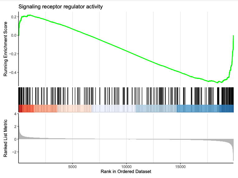
→ Provide the ranked gene list to GSEA. The rank is ordered from the largest Log2FC to smallest Log2FC. Therefore, since largest Log2FC represents upregulation in KO (treatment sample), the left side of GSEA plot is KO, while the right side of the plot is WT.

C5 GSEA

GSEA.C5.KOvsWT <- clusterProfiler::GSEA(LFC.KOvsWT,
                                             TERM2GENE = MSigDb.human.c5,
                                             minGSSize = 10,
                                             maxGSSize = 800,
                                             pvalueCutoff = 1,
                                             pAdjustMethod = "fdr",
                                             by = "fgsea")
# filter
GSEA.C5.KOvsWT_filter <-
clusterProfiler::filter(GSEA.C5.KOvsWT,
                        p.adjust < 0.05,
                        qvalue < 0.1,
                        abs(NES)>1)

GSEA.C5.KOvsWT_filter <- GSEA.C5.KOvsWT_filter %>% arrange(p.adjust)


write.csv(GSEA.C5.KOvsWT_filter@result,
          file="###",
          row.names = FALSE,
          quote = FALSE)

GSEA.C5.KOvsWT_filter@result

GSEA.C5.KOvsWT_filter@result$ONTOLOGY <-
                        gsub("_.*", "", GSEA.C5.KOvsWT_filter@result$ID)

Dotplot

showCategory <- GSEA.C5.KOvsWT_filter@result$ID[1:10]

pdf(file = "###")
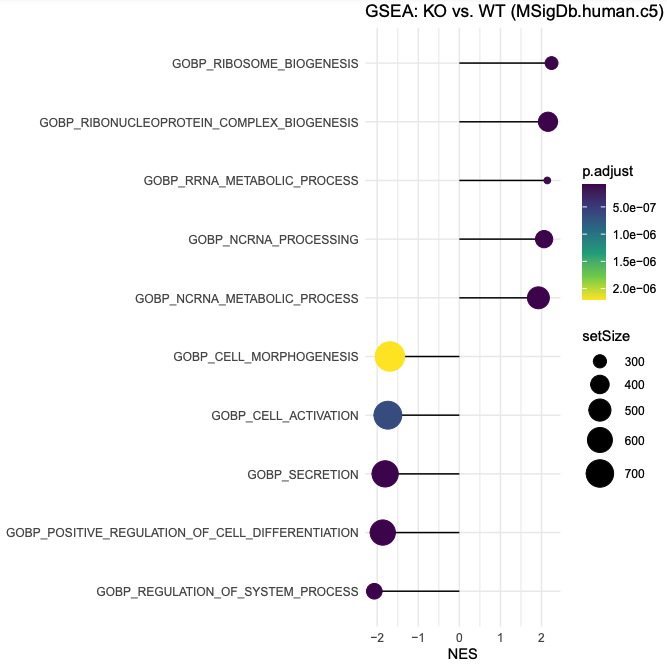
ggplot(GSEA.C5.KOvsWT_filter, showCategory = GSEA.C5.KOvsWT_filter@result$ID[1:10],
  aes(NES, forcats::fct_reorder(Description, NES))) +
  geom_segment(aes(xend=0, yend = Description)) +
  geom_point(aes(color=p.adjust, size = setSize)) +
  scale_color_viridis_c(guide=guide_colorbar(reverse=TRUE)) +
  scale_size_continuous(range=c(2, 10)) +
  theme_minimal() +
  xlab("NES") +
  ylab(NULL) +
  ggtitle("GSEA: KO vs. WT (MSigDb.human.c5)")
dev.off()

Cnetplot

pdf(file = "###", width = 10, height = 7)
enrichplot::cnetplot(GSEA.C5.KOvsWT_filter,
                     circular=F,
                     color.params = list(foldChange = LFC.KOvsWT, edge = TRUE),
                     cex.params = list(category_label = 0.5),
                     showCategory = 4,
                     cex_line = 0.5,
                     node_label="category")+
  ggtitle("GSEA: KO vs. WT (MSigDb.human.c5)")
dev.off()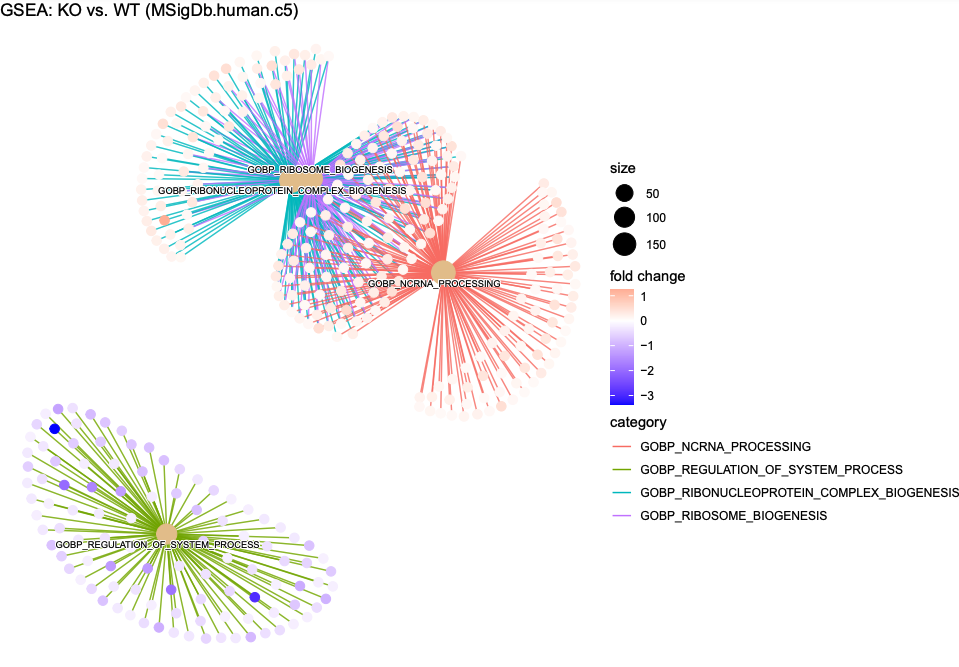

Ridgeplot

The ridgeplot will visualize expression distributions of core enriched genes for GSEA enriched categories. It helps users to interpret up/down-regulated pathways.

pdf(file = "###")
ridgeplot(GSEA.C5.KOvsWT_filter,
          showCategory = 10)+
  ggtitle("GSEA: KO vs. WT (MSigDb.human.c5)")
dev.off()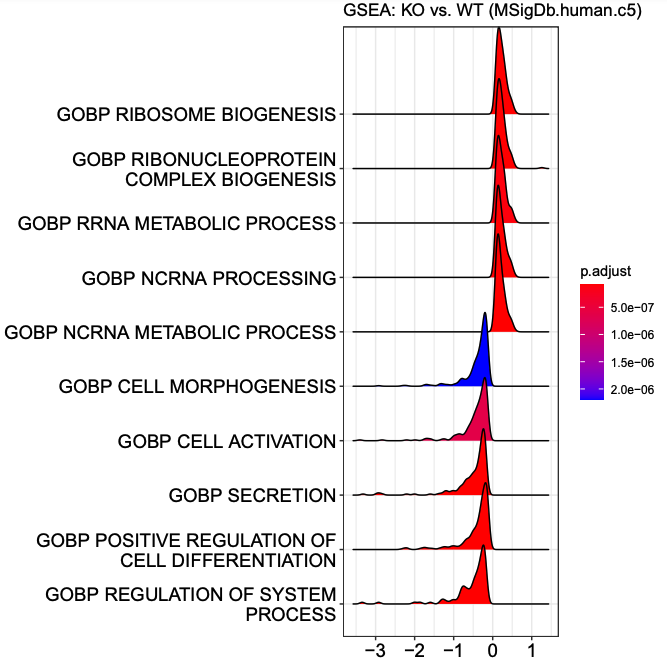

**Certain GSEA plot (SIGNALING_RECEPTOR_REGULATOR_ACTIVITY)**

grep("SIGNALING_RECEPTOR_REGULATOR_ACTIVITY", GSEA.C5.KOvsWT_filter@result$ID, ignore.case = TRUE) # 64

pdf(file = "GSEAplot_SIGNALING_RECEPTOR_REGULATOR_ACTIVITY.pdf", width = 8, height = 6)
enrichplot::gseaplot2(GSEA.C5.KOvsWT_filter, 
          geneSetID = 64, 
          title = "Signaling receptor regulator activity")
dev.off()

← Back to projects