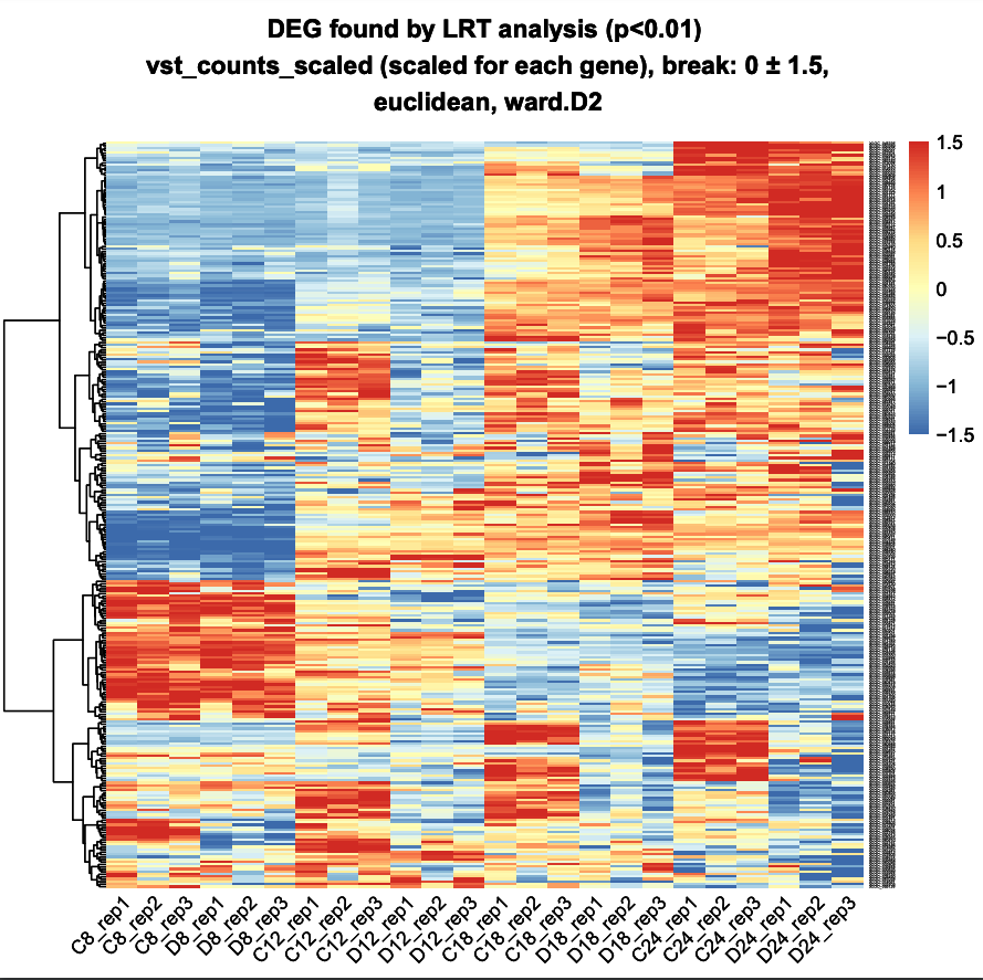
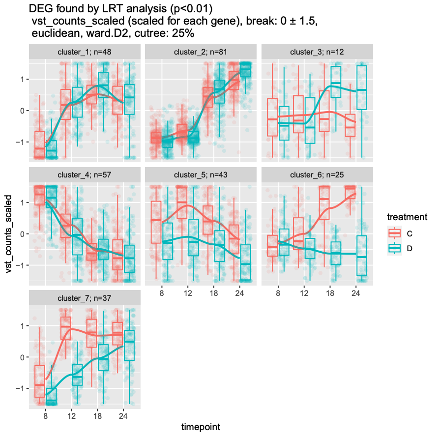
In this page we change the workflow to “split the dds object for each timepoint”. And please note that the RNAseq data of Pdu was subsetted with only LONGEST isoform left defined with “extract_isoform” pipeline. Not all genes in RNAseq data were involved in analysis.
Why SPLIT?
In this kind of data, we see that difference between samples in** timepoint 8** is smaller than other timepoints. For these data, one dispersion parameter per gene did not adequately reflect the differences between time points. I therefore separated the time points when creating the dds objects.
Comparing the standard and split DESeq2 workflows
I compared the following two workflows.
1. Pairwise comparisons in the standard DESeq2 workflow
Normalize using a shared model, then use a contrast to extract the two groups of interest.
2) split data pipeline
First subset the two groups of interest, then normalize them with their own model. This produces separate models for the individual comparisons.
D8 vs C8
8 timepoint (standard pipeline) → 27 DEGs 8 timepoint (split pipeline) → 85 DEGs
ggvenn(list('Std_pipeline_DEG_8' = result_D8_C8_shrink_df_subset.pvalue$Gene,
            'Split_pipeline_DEG_8' = new_result_D8_C8_shrink_df_subset.pvalue$Gene),
       c("Std_pipeline_DEG_8",
         "Split_pipeline_DEG_8"))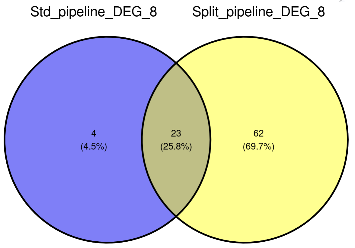
D12 vs C12
12 timepoint (standard pipeline) → 147 DEGs 12 timepoint (split pipeline) → 134 DEGs
ggvenn(list('Std_pipeline_DEG_12' = result_D12_C12_shrink_df_subset.pvalue$Gene,
'Split_pipeline_DEG_12' = new_result_D12_C12_shrink_df_subset.pvalue$Gene),
c("Std_pipeline_DEG_12",
"Split_pipeline_DEG_12"))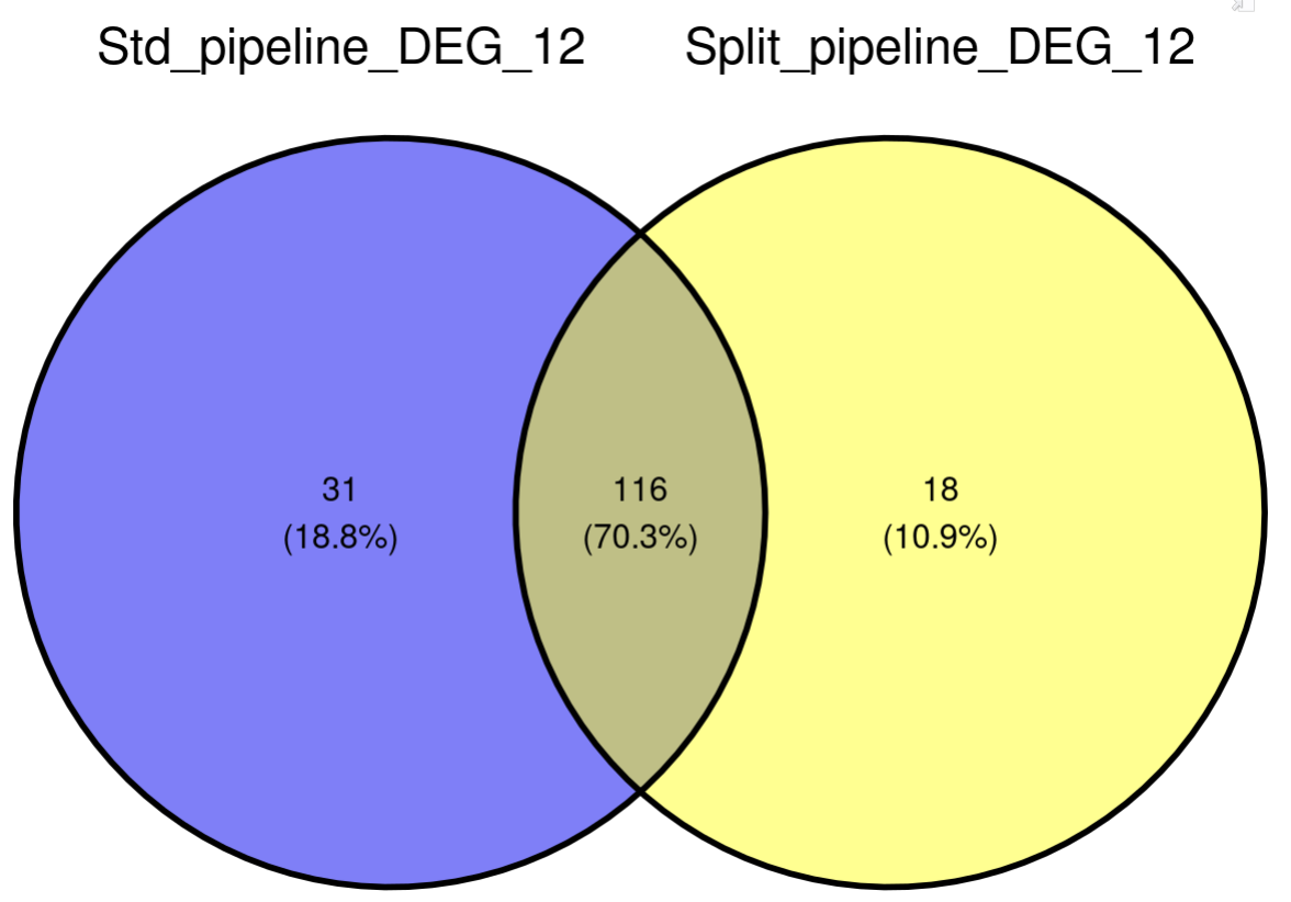
D18 vs C18
18 timepoint (standard pipeline) → 87 DEGs 18 timepoint (split pipeline) → 86 DEGs
ggvenn(list('Std_pipeline_DEG_18' = result_D18_C18_shrink_df_subset.pvalue$Gene,
            'Split_pipeline_DEG_18' = new_result_D18_C18_shrink_df_subset.pvalue$Gene),
       c("Std_pipeline_DEG_18",
         "Split_pipeline_DEG_18"))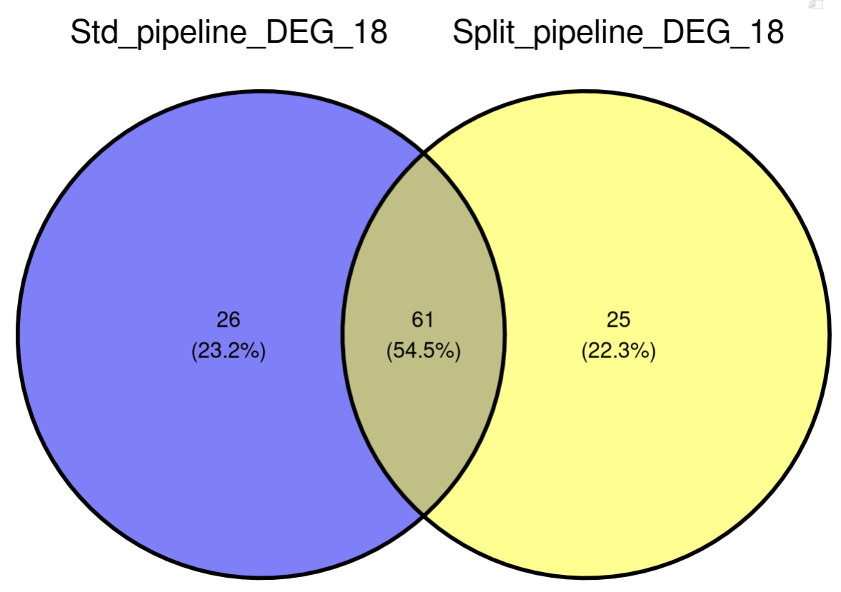
D24 vs C24
24 timepoint (standard pipeline) → NO DEGs if we did not perform prefiltering 24 timepoint (split pipeline) → 86 DEGs
ggvenn(list('Std_pipeline_DEG_24' = result_D24_C24_shrink_df_subset.pvalue$Gene,
            'Split_pipeline_DEG_24' = new_result_D24_C24_shrink_df_subset.pvalue$Gene),
       c("Std_pipeline_DEG_24",
         "Split_pipeline_DEG_24"))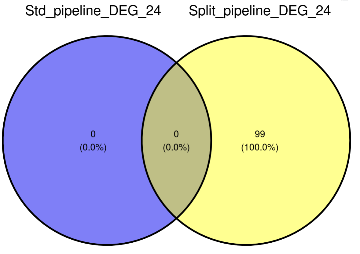
Workflow:
Steps:
- Subset genes based on the result of extract_isoform
- Pairwise comparison (no pre-filtering); SPLIT the dds object for each time point
- Pairwise comparison: clustering
- LRT analysis
- LRT clustering
Example:
Library and Data Import
setwd("###")

library(DESeq2)
library(ashr)
library(ggvenn)    # for Venn Diagram
library(car)  # point labels without overlaps
library(umap) # umap
# input the tab-delimited text file of count matrix
count_matrix <- read.table("count_matrix.txt",
header = TRUE,
row.names = 1,
sep = "\t",
check.names = F)
count_matrix_raw <- count_matrix[,c(7:30)]
write.csv(count_matrix_raw, file = "Raw_counts.csv")
metadata <- read.table("metadata.txt",
header = TRUE,
row.names = 1,
sep = "\t",
check.names = F)
metadata$group <- factor(metadata$group, levels = c("C8","C12","C18","C24",
"D8","D12","D18","D24"))
metadata$rep <- factor(metadata$rep)
metadata$treatment <- factor(metadata$treatment)
metadata$timepoint <- factor(metadata$timepoint)
#################################################
####### Gene-Uniport_ID transformatiion ######### not necessary
#################################################
GeneID_metadata <- read.delim("###", header=FALSE, na.strings="N/A")
GeneID_metadata_BBH <- GeneID_metadata[GeneID_metadata$V5 == "BBH",] # 64548 -> 14216
GeneID_metadata_BBH <- GeneID_metadata_BBH[,c(1,4)]
colnames(GeneID_metadata_BBH) = c("Gene", "Uniport_ID")
##########################################################
####### gene list after extract_isoform pipeline #########
##########################################################
gene_list_extract_isoform <- read_delim("###",
delim = "\t", escape_double = FALSE,
col_names = FALSE, trim_ws = TRUE)
TF_list_Intersection <- "///Intersection_Pdu.AnimalTFDB4.0_Pdu.BH.txt"
TF_list_Union <- "///Union_Pdu.AnimalTFDB4.0_Pdu.BH.txt"colnames(count_matrix_raw) <- c("C12_rep1",
"C12_rep2",
"C12_rep3",
"C18_rep1",
"C18_rep2",
"C18_rep3",
"C24_rep1",
"C24_rep2",
"C24_rep3",
"C8_rep1",
"C8_rep2",
"C8_rep3",
"D12_rep1",
"D12_rep2",
"D12_rep3",
"D18_rep1",
"D18_rep2",
"D18_rep3",
"D24_rep1",
"D24_rep2",
"D24_rep3",
"D8_rep1",
"D8_rep2",
"D8_rep3")
count_matrix_raw <- count_matrix_raw[, c("C8_rep1", "C8_rep2","C8_rep3",
"D8_rep1", "D8_rep2","D8_rep3",
"C12_rep1","C12_rep2","C12_rep3",
"D12_rep1","D12_rep2","D12_rep3",
"C18_rep1","C18_rep2","C18_rep3",
"D18_rep1","D18_rep2","D18_rep3",
"C24_rep1","C24_rep2","C24_rep3",
"D24_rep1","D24_rep2","D24_rep3")]Subset genes based on the result of extract_isoform:
# eliminate rows with NAs
count_matrix_raw <- na.omit(count_matrix_raw)
# 69611 -> 69611 no change

# are there duplicated geneID?
length(unique(rownames(count_matrix_raw)))
# no

# Subset only genes after extract_isoform pipeline
count_matrix_extract_isoform <- count_matrix_raw[rownames(count_matrix_raw) %in% gene_list_extract_isoform$X1,]
Output cross-sample normalized matrix
dds <- DESeqDataSetFromMatrix(countData= count_matrix_extract_isoform,
                              colData= metadata,
                              design= ~group+rep)

# Size factor
dds<-estimateSizeFactors(dds)

normalized_counts <- counts(dds, normalized=TRUE)
normalized_counts <- tibble::rownames_to_column(as.data.frame(normalized_counts), "Gene")

write.csv(normalized_counts, file = "DESeq2_cross-sample_normalized_counts.csv")
vst <- vst(dds, blind=FALSE)
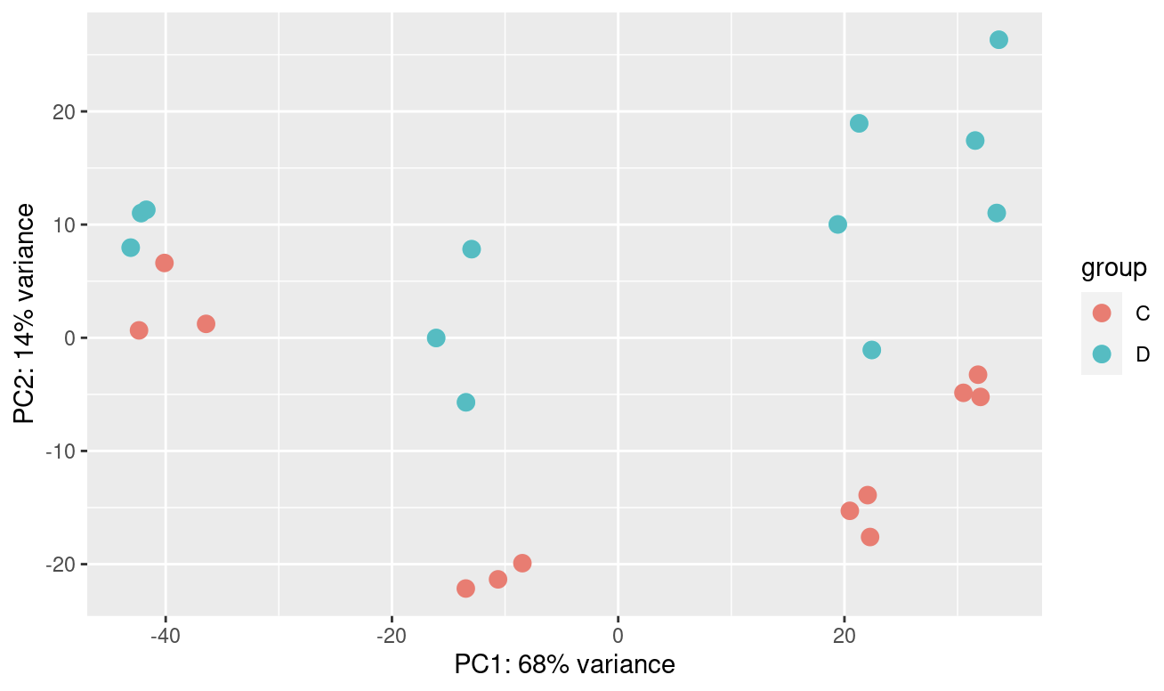
plotPCA(vst,intgroup="group")
plotPCA(vst,intgroup="treatment")
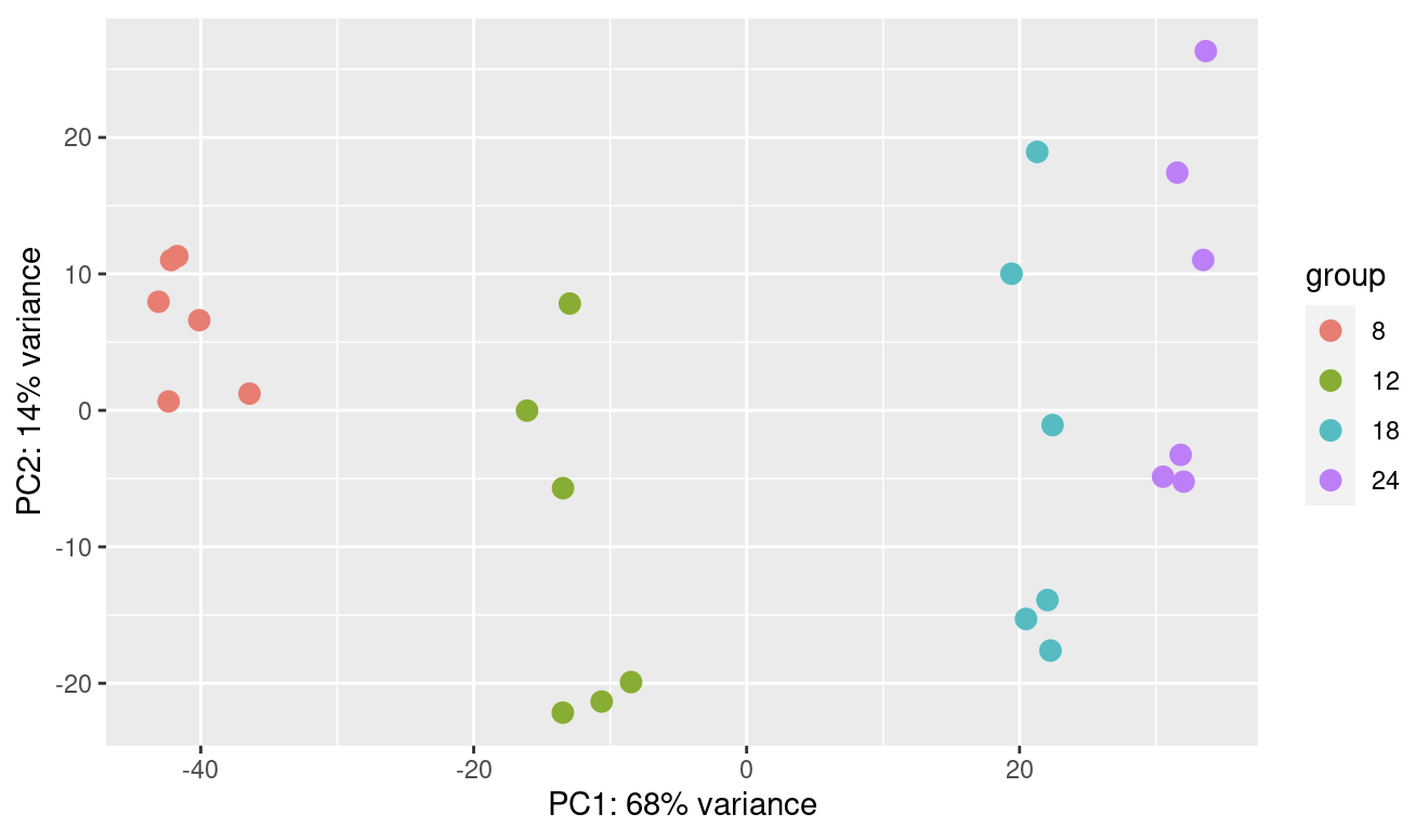
plotPCA(vst,intgroup="timepoint")
plotPCA(vst,intgroup="rep")
vst_mat <- assay(vst)
write.csv(vst_mat, file = "DESeq2_cross-sample_normalized_vst-counts.csv")Pairwise comparison (no pre-filtering); SPLIT the dds object for each time point
D8 vs C8
subset “8” timepoint
count_matrix_raw_8 <- subset(count_matrix_extract_isoform,
                             select = grepl("C8|D8",names(count_matrix_extract_isoform)))

metadata_8 <- metadata[metadata$timepoint == "8",]
metadata_8$group <- factor(metadata_8$group, levels = c("C8","D8"))
metadata_8$timepoint <- factor(metadata_8$timepoint, levels = c("8"))


dds_8 <- DESeqDataSetFromMatrix(countData= count_matrix_extract_isoform_8,
                              colData= metadata_8,
                              design= ~group+rep)
dds_wald_8 <- DESeq(dds_8,
test = "Wald",
fitType = "parametric",
betaPrior = F) # whether or not to put a zero-mean normal prior on the non-intercept coefficients
summary(results(dds_wald_8))
plotDispEsts(dds_wald_8)out of 23706 with nonzero total read count
adjusted p-value < 0.1
LFC > 0 (up) : 2978, 13%
LFC < 0 (down) : 3057, 13%
outliers [1] : 0, 0%
low counts [2] : 7277, 31%
(mean count < 3)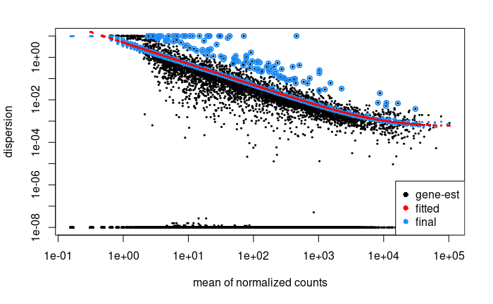
result_D8_C8 <-results(dds_wald_8,
                      contrast=c("group","D8","C8"), # base factor level 放後面
                      alpha = 0.05,
                      lfcThreshold = 0, # default
                      independentFiltering = TRUE,
                      pAdjustMethod = "fdr")
# (genes' logFC > 0 表示 genes are overexpressed in D8 group)


result_D8_C8_df <- as.data.frame(result_D8_C8)
result_D8_C8_df <- result_D8_C8_df[order(result_D8_C8_df$padj),]

write.csv(result_D8_C8_df, file = "###")

# check if any genes has baseMean = 0?
result_D8_C8_df[result_D8_C8_df$baseMean == 0,]
# 4717 genes

# check if there are any outlier: pvalue and padj = NA?
result_D8_C8_df[is.na(result_D8_C8_df$pvalue) & is.na(result_D8_C8_df$padj),]
# -> 有 4717 個 genes 是 outlier

# check how many genes were filtered by automatic independent filtering, for having a low mean normalized count: only padj = NA?
result_D8_C8_df[is.na(result_D8_C8_df$padj) & !is.na(result_D8_C8_df$pvalue),]
# -> 有 8641 個 genes 被 independent filtered

metadata(result_D8_C8)$filterThreshold- DESeq2 has filtered out genes with a mean count of
4.304395. As a result,46.99738% of genes were filtered out of the analysis
# "ashr"
result_D8_C8_shrink_ashr <- lfcShrink(dds_wald_8,
                                      type="ashr",
                                      res = result_D8_C8)

plotMA(result_D8_C8)
# If you see a lot of variability or small fold changes, "apeglm" might be more appropriate. If there is a trend of variance changing with average expression, "ashr" could be a good choice.

plotMA(result_D8_C8_shrink_ashr)


############################
# -> ashr seems to be better
result_D8_C8_shrink_ashr_df <- as.data.frame(result_D8_C8_shrink_ashr)
result_D8_C8_shrink_ashr_df <- result_D8_C8_shrink_ashr_df[order(result_D8_C8_shrink_ashr_df$padj),]


write.csv(result_D8_C8_shrink_ashr_df, file = "###")
before lfcShrink vs after
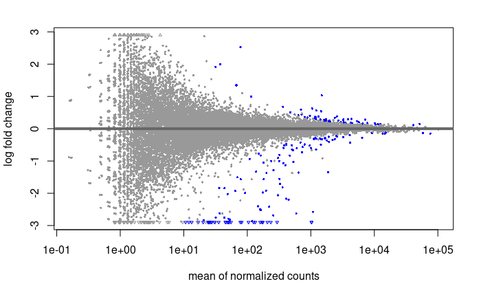
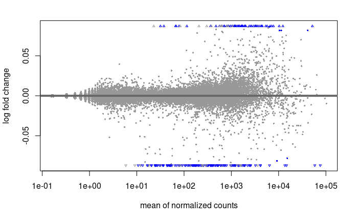
DEG subset (pvalue < 0.01; abs(logFC) > 1)
#############################################################
######### pvalue < 0.01; abs(logFC) > 1 ##################
#############################################################
result_D8_C8_shrink_df_subset.pvalue <- subset(result_D8_C8_shrink_ashr_df,
                                 (result_D8_C8_shrink_ashr_df$pvalue < 0.01 &
                                  abs(result_D8_C8_shrink_ashr_df$log2FoldChange) > 1))


result_D8_C8_shrink_df_subset.pvalue <- tibble::rownames_to_column(result_D8_C8_shrink_df_subset.pvalue, "Gene")
# -> 70 DEGs

# 插入 cross-sample normalized counts
result_D8_C8_shrink_df_subset.pvalue <- merge(result_D8_C8_shrink_df_subset.pvalue,
                                            subset(normalized_counts,
                                                   select = grepl("Gene|C8|D8",
                                                                  names(normalized_counts))),
                                            by = "Gene")
result_D8_C8_shrink_df_subset.pvalue <- merge(result_D8_C8_shrink_df_subset.pvalue,
                                            GeneID_metadata_BBH,
                                            by = "Gene",
                                            all = T)
result_D8_C8_shrink_df_subset.pvalue <- result_D8_C8_shrink_df_subset.pvalue[!is.na(result_D8_C8_shrink_df_subset.pvalue$baseMean),]


# 這邊會有同樣 geneID 但不同 UniportID的出現在表格中

#移除重複的 rows,留下編號小的uniportID
# 例如:
# XLOC_005048 .... 10096|comp215221_c2_seq1|ID4_XENTR
# XLOC_005048 .... 10097|comp215221_c2_seq10|ID2_XENTR
# 要留下 10096|comp215221_c2_seq1|ID4_XENTR 這一個 row 就好
# 所以先根據 uniportID 排序
result_D8_C8_shrink_df_subset.pvalue <- result_D8_C8_shrink_df_subset.pvalue[order(result_D8_C8_shrink_df_subset.pvalue$Uniport_ID),]

# 移除重複的 rows
result_D8_C8_shrink_df_subset.pvalue <- result_D8_C8_shrink_df_subset.pvalue[!duplicated(result_D8_C8_shrink_df_subset.pvalue$Gene),]


write.csv(result_D8_C8_shrink_df_subset.pvalue,
          file = "###")
volcano plot
volcano_D8_C8_shrink_ashr_df <- result_D8_C8_shrink_ashr_df


volcano_D8_C8_shrink_ashr_df$shape <- ifelse(volcano_D8_C8_shrink_ashr_df$pvalue<10^-55,
                                            2,
                                            20)
volcano_D8_C8_shrink_ashr_df$pvalue[volcano_D8_C8_shrink_ashr_df$pvalue<10^-55] <- 10^-55


pdf(file = "split_dds/volcano_D8vsC8.pdf", height = 5, width = 7)
# Make a basic volcano plot
with(volcano_D8_C8_shrink_ashr_df,
     plot(log2FoldChange,
          -log10(pvalue),
          pch=shape,
          main="Volcano plot: D8 vs C8 (base); lfcShrink (ashr)"))

# Add colored points: blue if log2FC < -1 and pvalue < 0.01
# red if log2FC > 1 and padj<0.05)
with(subset(volcano_D8_C8_shrink_ashr_df,
            pvalue<.01 & log2FoldChange < -1),
     points(log2FoldChange,
            -log10(pvalue),
            pch=shape,
            col="blue"))

with(subset(volcano_D8_C8_shrink_ashr_df,
            pvalue<.01 & log2FoldChange > 1),
     points(log2FoldChange,
            -log10(pvalue),
            pch=shape,
            col="red"))

legend("topright",
       legend=c("log2FC < -1 and pvalue < 0.01",
                "log2FC > 1 and pvalue < 0.01"),
       col=c("blue", "red"),
       cex = 0.6,
       pch = 20)
dev.off()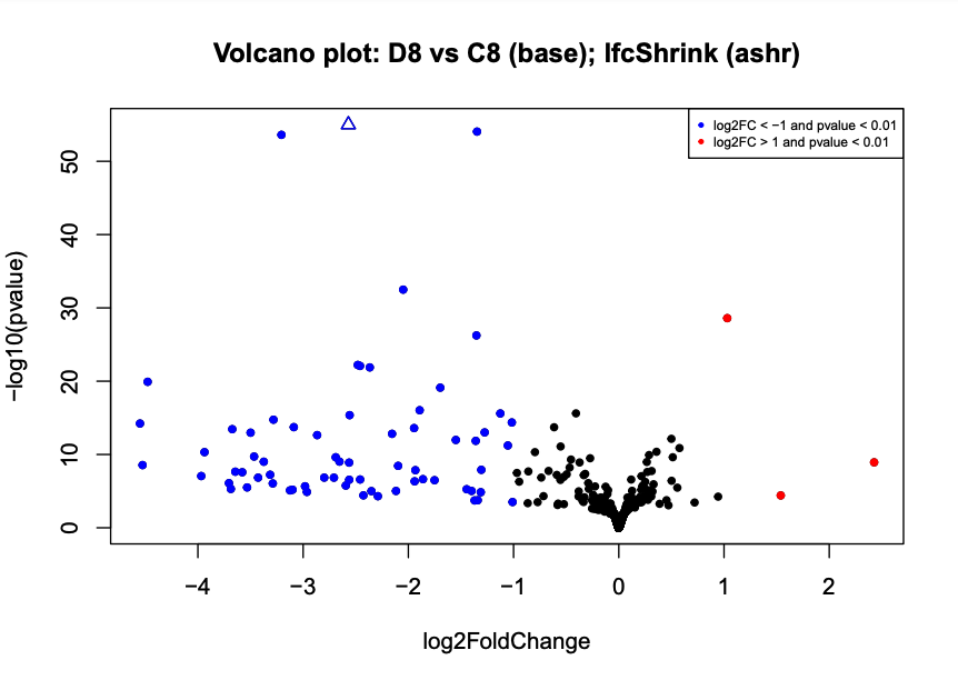
D12 vs C12 (same as above)
D18 vs C18 (same as above)
C24 vs D24 (same as above)
Pairwise comparison: clustering
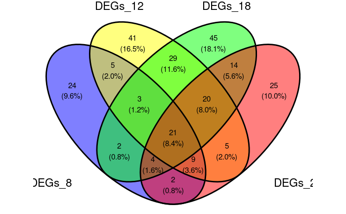
Compare DEG overlap across the four pairwise contrasts
result_D8_C8_shrink_df_subset.pvalue
result_D12_C12_shrink_df_subset.pvalue
result_D18_C18_shrink_df_subset.pvalue
result_D24_C24_shrink_df_subset.pvalue
ggvenn(list("DEGs_8" = result_D8_C8_shrink_df_subset.pvalue$Gene,
            "DEGs_12" = result_D12_C12_shrink_df_subset.pvalue$Gene,
            "DEGs_18" = result_D18_C18_shrink_df_subset.pvalue$Gene,
            "DEGs_24" = result_D24_C24_shrink_df_subset.pvalue$Gene),
       c("DEGs_8",
         "DEGs_12",
         "DEGs_18",
         "DEGs_24"))
The combined set contained 249 genes.
Visualization (using vstHeatmapWithClustering helper function)
DEGs_all <- unique(
            c(result_D8_C8_shrink_df_subset.pvalue$Gene,
              result_D12_C12_shrink_df_subset.pvalue$Gene,
              result_D18_C18_shrink_df_subset.pvalue$Gene,
              result_D24_C24_shrink_df_subset.pvalue$Gene))

vst_DEGs_all <- vst_mat[rownames(vst_mat) %in% DEGs_all,]

source("###")


pdf(file = "###")
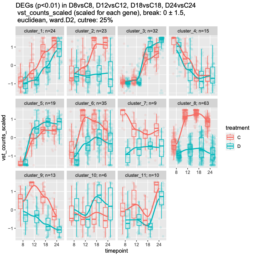
heatmap_and_clusterPattern(matrix = vst_DEGs_all,
                           heatmap_title = "DEGs (p<0.01) in D8vsC8, D12vsC12, D18vsC18, D24vsC24\n vst_counts_scaled (scaled for each gene), break: 0 \u00b1 1.5,\n euclidean, ward.D2",
                           value_break = 1.5,
                           PatternCluster = T,
                           PatternCluster_csv.file = "split_dds/cluster_results.csv",
                           PatternCluster_txt.file = "split_dds/cluster_results.txt",
                           PatternCluster_title = "DEGs (p<0.01) in D8vsC8, D12vsC12, D18vsC18, D24vsC24\n vst_counts_scaled (scaled for each gene), break: 0 \u00b1 1.5,\n euclidean, ward.D2, cutree: 25%")
dev.off()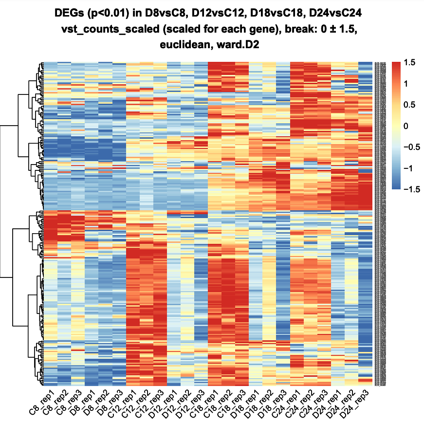
LRT analysis
- treatment difference at time 0
- the difference over time
- and any treatment-specific differences over time (the interaction term)
dds_time <- DESeqDataSetFromMatrix(countData= count_matrix_extract_isoform,
                                   colData= metadata,
                                   design= ~treatment + timepoint + treatment:timepoint + rep)

# Size factor
dds_time<-estimateSizeFactors(dds_time)

normalized_counts <- counts(dds_time, normalized=TRUE)
normalized_counts <- tibble::rownames_to_column(as.data.frame(normalized_counts), "Gene")

write.csv(normalized_counts, file = "LRT-DESeq2_cross-sample_normalized_counts.csv")


vst <- vst(dds_time, blind=FALSE)

plotPCA(vst,intgroup="group")
plotPCA(vst,intgroup="treatment")
plotPCA(vst,intgroup="timepoint")
plotPCA(vst,intgroup="rep")

vst_mat <- assay(vst)
write.csv(vst_mat, file = "LRT-DESeq2_cross-sample_normalized_vst-counts.csv")
dds_time_LRT <- DESeq(dds_time,
test="LRT",
reduced = ~ treatment + timepoint + rep)
summary(results(dds_time_LRT))
plotDispEsts(dds_time_LRT)out of 26049 with nonzero total read count
adjusted p-value < 0.1
LFC > 0 (up) : 98, 0.38%
LFC < 0 (down) : 69, 0.26%
outliers [1] : 0, 0%
low counts [2] : 10052, 39%
(mean count < 3)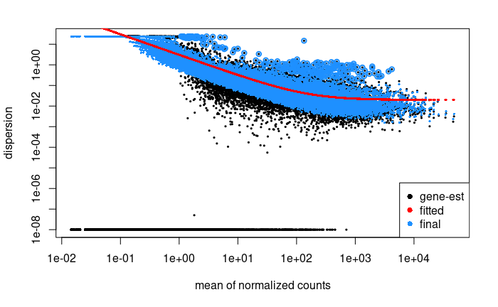
# now log2FC is treatmentD.timepoint24 (very difficult to explain)
# By default, the result() function will return the LRT test p-value and MLE log2FC for the difference between Mut vs WT at the last timepoints, controlling for baseline
# no matter what the "name =" argument is, baseMean, pvalue and padj never change!!
result_time <- results(dds_time_LRT,
                        name = "treatmentD.timepoint24",
                        pAdjustMethod = "fdr",
                        independentFiltering = TRUE,
                        alpha = 0.05)


result_time_df <- as.data.frame(result_time)
result_time_df <- result_time_df[order(result_time_df$padj),]


write.csv(result_time_df, file = "//deseq2_result.csv")

# check if any genes has baseMean = 0?
result_time_df[result_time_df$baseMean == 0,]
# 2374 genes

# check if there are any outlier: pvalue and padj = NA?
result_time_df[is.na(result_time_df$pvalue) & is.na(result_time_df$padj),]
# -> 有 2374 個 gene 是 outlier

# check how many genes were filtered by automatic independent filtering, for having a low mean normalized count: only padj = NA?
result_time_df[is.na(result_time_df$padj) & !is.na(result_time_df$pvalue),]
# -> 有 10052 個 gene 被 independent filtered

metadata(result_time)$filterThreshold- DESeq2 has filtered out genes with a mean count of
2.774961. As a result,43.71876% of genes were filtered out of the analysis
#############################################################
######### pvalue < 0.01 #####################################
#############################################################
result_time_df_subset.pvalue <- subset(result_time_df,
                                 (result_time_df$pvalue < 0.01))


result_time_df_subset.pvalue <- tibble::rownames_to_column(result_time_df_subset.pvalue, "Gene")
# -> 303 DEGs


result_time_df_subset.pvalue <- merge(result_time_df_subset.pvalue,
                                      normalized_counts,
                                      by = "Gene")

result_time_df_subset.pvalue <- merge(result_time_df_subset.pvalue,
                                            GeneID_metadata_BBH,
                                            by = "Gene",
                                            all = T)
result_time_df_subset.pvalue <- result_time_df_subset.pvalue[!is.na(result_time_df_subset.pvalue$baseMean),]


# 這邊會有同樣 geneID 但不同 UniportID的出現在表格中

#移除重複的 rows,留下編號小的uniportID
# 所以先根據 uniportID 排序
result_time_df_subset.pvalue <- result_time_df_subset.pvalue[order(result_time_df_subset.pvalue$Uniport_ID),]

# 移除重複的 rows
result_time_df_subset.pvalue <- result_time_df_subset.pvalue[!duplicated(result_time_df_subset.pvalue$Gene),]


write.csv(result_time_df_subset.pvalue,
          file = "//DEGs_LRT_pvalue<0.01.csv")
LRT clustering
# subset only DEGs (pvalue < 0.01)
vst_sig <- vst_mat[rownames(vst_mat) %in% result_time_df_subset.pvalue$Gene,]


pdf(file = "LRT_analysis/hmap_LRT.DEGs_p<0.01_vst.scale.pdf")
heatmap_and_clusterPattern(matrix = vst_sig,
                           heatmap_title = "DEG found by LRT analysis (p<0.01)\n vst_counts_scaled (scaled for each gene), break: 0 \u00b1 1.5,\n euclidean, ward.D2",
                           value_break = 1.5,
                           PatternCluster = T,
                           PatternCluster_csv.file = "LRT_analysis/cluster_results.csv",
                           PatternCluster_txt.file = "LRT_analysis/cluster_results.txt",
                           PatternCluster_title = "DEG found by LRT analysis (p<0.01)\n vst_counts_scaled (scaled for each gene), break: 0 \u00b1 1.5,\n euclidean, ward.D2, cutree: 25%")
dev.off()