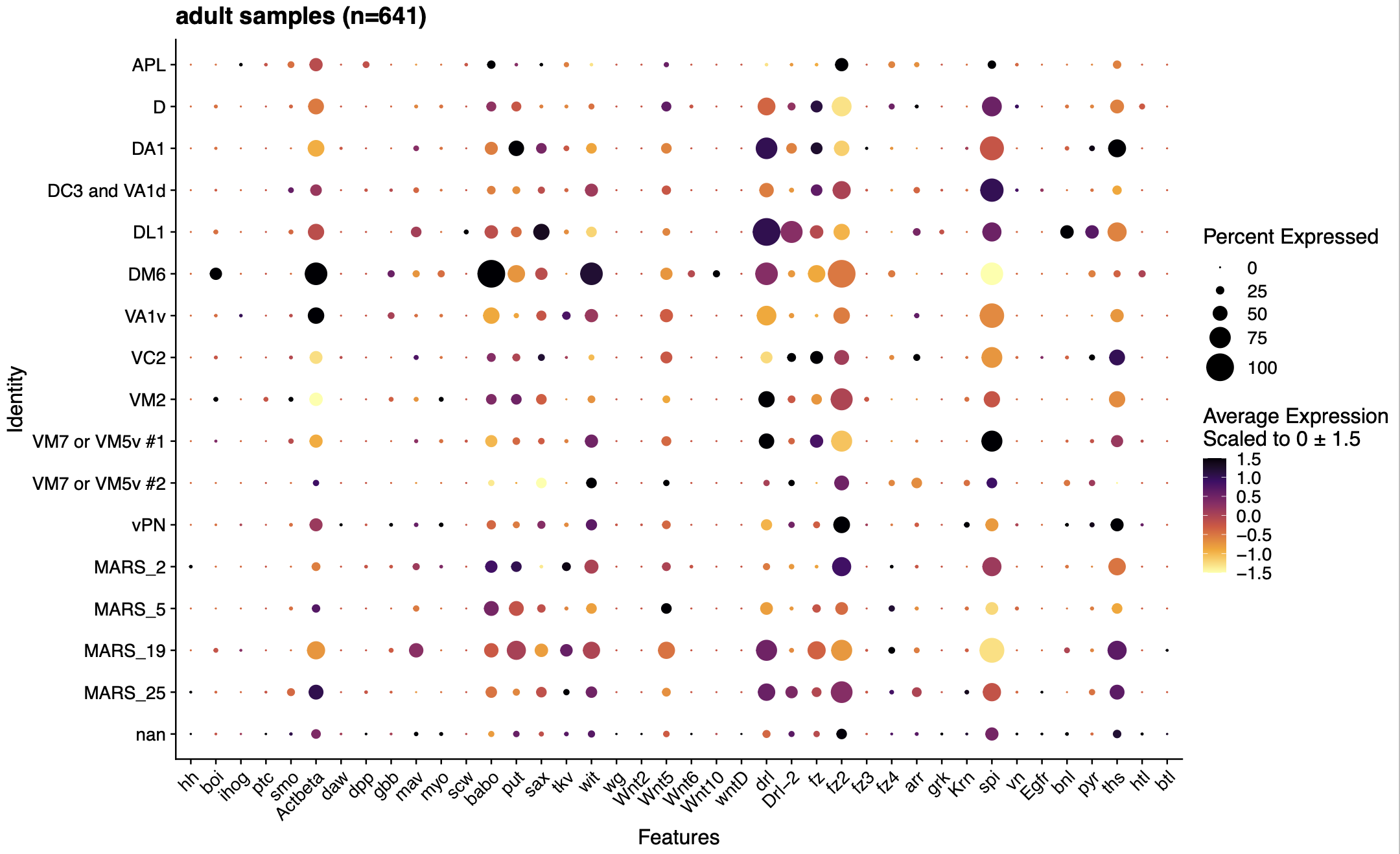
The DotplotNN function defines a dot-plot visualization. Its implementation, example call, and recorded output are presented together below.
DotplotNN function
DotPlotNN <- function(object, assay = NULL, features, cols = c("lightgrey", "blue"), viridis_type = "D", viridis_direction = -1, col.min = -2.5, col.max = 2.5, dot.min = 0, dot.scale = 6, idents = NULL, group.by = NULL, scale = TRUE, scale.by = "radius", scale.min = NA, scale.max = NA) {


  # Define function PercentAbove for calculating percentage expression of each feature
  PercentAbove <- function(x, threshold) {
    return(length(x[x > threshold]) / length(x))
  }
  # Retrieve the assay
  assay <- assay %||% DefaultAssay(object)
  DefaultAssay(object) <- assay


  # define "scale" function based on the argument "scale.by"
  scale.func <- switch(EXPR = scale.by,
                       size = scale_size, # if "scale.by=size" -> use "scale_size"
                       radius = scale_radius,  # if "scale.by=radius" -> use "scale_radius"
                       stop("\'scale.by\' must be either \'size\' or \'radius\'"))


  # Tidy the features
  feature.groups <- NULL
  # if the features provided is a LIST
  if (is.list(features) | any(!is.na(names(features)))) {
      # assign group name to each feature
      feature.groups <- unlist(
                        sapply(X = 1:length(features), FUN = function(x) {
        return(rep(names(features)[x], each = length(features[[x]])))
      })
      )

      if (any(is.na(x = feature.groups))) {
        warning("Some feature groups are unnamed.", call. = FALSE, immediate. = TRUE)
      }

      features <- unlist(x = features)
      names(feature.groups) <- features
  }


  # Retrieve cell ID
  cells <- unlist(CellsByIdentities(object, idents))
  # Retrieve the count matrix (row x column: cell ID x features)
  data.features <- FetchData(object, vars = features, cells = cells)

  # If group.by=NULL, assign active.ident as cell ID
  # Here normally I either already assign celltypes as active.ident before, or use group.by="celltypes"
  data.features$id <- if (is.null(x = group.by)) {
    Idents(object)[cells, drop = TRUE]
  } else {
    object[[group.by, drop = TRUE]][cells, drop = TRUE]
  }

  # if the ID column is not a factor variable:
  if (!is.factor(x = data.features$id)) {
    data.features$id <- factor(x = data.features$id)
  }

  # Retrieve the ID levels and convert ID column back to characters:
  id.levels <- levels(x = data.features$id)
  data.features$id <- as.vector(x = data.features$id)


  data.plot <- lapply(X = unique(data.features$id), FUN = function(X) {
            # Retrieve the count matrix of certain celltype
            data.use <- data.features[data.features$id == X, 1:(ncol(data.features) - 1), drop = FALSE]

            # Calculate the avg expression of each feature (apply by column)
            avg.exp <- apply(data.use, MARGIN = 2, FUN = function(x) {
            return(mean(x))
            })

            # Calculate the percentage expression of each feature (apply by column)
            pct.exp <- apply(X = data.use, MARGIN = 2, FUN = PercentAbove, threshold = 0)
            return(list(avg.exp = avg.exp, pct.exp = pct.exp))
  })
  names(data.plot) <- unique(x = data.features$id)

  # Add 2 object in each list: feature name and celltype ID
  data.plot <- lapply(X = names(data.plot), FUN = function(x) {
            data.use <- as.data.frame(data.plot[[x]])
            data.use$features.plot <- rownames(data.use)
            data.use$id <- x
            return(data.use)
  })

  # rbind all list together
  data.plot <- do.call(what = "rbind", args = data.plot)

  # Assign levels for the celltypes
  if (!is.null(id.levels)) {
    data.plot$id <- factor(data.plot$id, levels = id.levels)
  }
  if (length(levels(data.plot$id)) == 1) {
    scale <- FALSE
    warning("Only one identity present, the expression values will be not scaled", call. = FALSE, immediate. = TRUE)
  }


  #######################
  ### scale the data  ###
  #######################
  # In each feature, we scale it, so you can better visualize the difference of a gene between celltypes
  # But you may NOT compare difference of genes within a celltype
  avg.exp.scaled <- sapply(X = unique(data.plot$features.plot), FUN = function(x) {

            data.use <- data.plot[data.plot$features.plot == x, "avg.exp"]
            if (scale) {
                  data.use <- scale(data.use)
                  # convert to min < x < max
                  data.use <- MinMax(data = data.use, min = col.min, max = col.max)
            }
            return(data.use)
  })
  avg.exp.scaled <- as.vector(t(avg.exp.scaled))

  data.plot$avg.exp.scaled <- avg.exp.scaled
  data.plot$features.plot <- factor(x = data.plot$features.plot, levels = features)


  # if the percentage expression < dot.min: convert to NA
  #data.plot$pct.exp[data.plot$pct.exp < dot.min] <- NA


  ####################################
  # Convert the percentage expression
  # 設定最高最小的 Percentage expression 值(if present)
  data.plot$pct.exp <- data.plot$pct.exp * 100
  if (!is.na(scale.min)) {
    data.plot[data.plot$pct.exp < scale.min, "pct.exp"] <- scale.min
  }
  if (!is.na(x = scale.max)) {
    data.plot[data.plot$pct.exp > scale.max, "pct.exp"] <- scale.max
  }

  # 加上 feature 的 groups (if present)
  if (!is.null(feature.groups)) {
    data.plot$feature.groups <- factor(feature.groups[data.plot$features.plot], levels = unique(feature.groups))
  }

  ####################################
  # Visualization
  plot <- ggplot(data.plot,
                 mapping = aes_string(x = "features.plot",
                                      y = "id")) +
          geom_point(mapping = aes_string(size = "pct.exp",
                                          color = "avg.exp.scaled")) +
          scale.func(range = c(0, dot.scale),
                     limits = c(scale.min, scale.max)) +
          theme(axis.title.x = element_blank(),
                axis.title.y = element_blank()) +
          guides(size = guide_legend(title = "Percent Expressed")) +
          labs(x = "Features",
               y = "Identity") +
          cowplot::theme_cowplot()

  # Visualize the feature group
  if (!is.null(x = feature.groups)) {
    plot <- plot +
            facet_grid(facets = `~`(feature.groups),
                       scales = "free_x",
                       space = "free_x",
                       switch = "x") +
            theme(panel.spacing = unit(x = 1, units = "lines"),
                  strip.background = element_blank(),
                  strip.placement = "outside",
                  text = element_text(size = 16) # adjust the base_size
                                                                                                                       )
  }

  # Color gradient of the average expression
  data_range <- range(data.plot$avg.exp.scaled, na.rm = TRUE)
  if (length(cols) == 1 && cols != c("viridis")) {

          plot <- plot + scale_color_distiller(palette = cols)

  } else if (length(cols) == 1 && cols == c("viridis")) {

          if (scale){
            plot <- plot + scale_color_viridis_c(option = viridis_type,
                                                 direction = viridis_direction,
                                                 breaks = c(data_range[1]+0.1, data_range[2]-0.1),
                                                 labels = c("low", "high"))
          } else {
            plot <- plot + scale_color_viridis_c(option = viridis_type,
                                                 direction = viridis_direction,
                                                 breaks = c(data_range[1]+0.5, data_range[2]-0.5),
                                                 labels = c("low", "high"))
          }

  } else {
    plot <- plot + scale_color_gradientn(colours = cols)
      }


  plot <- plot + guides(color = guide_colorbar(title = "Avg. Exp. Level"))
  return(plot)
}
Usage:
DotPlotNN(raw_seurat_Xie.adult,
                features = feature_list_symbol,
                dot.scale = 8,
                scale = TRUE,
                col.min = -1.5,
                col.max = 1.5,
                cols = c("viridis"),
                viridis_type = "B",
                viridis_direction = -1) +
                RotatedAxis() + ggtitle("adult samples (n=641)")