Regulon analysis with pySCENIC

My Notes

Before you do SCENIC analysis, think about →

1. Perform binarization in R or shell?
2. How to subset the regulons that you want to present on the heatmap?
   1. Filter out the regulons that express in cell number less than median(cell number).
   2. Perform FindMarkers() to obtain DE regulons.
   3. When we compare 2 condition of a celltype, which regulons should we need.
3. How do you arrange the order of regulons on the heatmap? hclust?

About this pipeline

1. We filter out the regulons that express in cell number less than median(cell number).
2. Perform binarization in R.
3. Pay attention on the gene order on heatmap.

In Shell

pySCENIC

pyscenic grn ./integrated_20230216.loom ./Mus_musculus_TF_SymbolOnly.txt -o adj.csv --num_workers 20

pyscenic ctx 
./adj.tsv 
~/Shared/mouse_lung_sc_rawData/SCENIC_20230213/Hajdarovic_workflow/RcisTarget_databases/*feather 
--annotations_fname motifs-v10nr_clust-nr.mgi-m0.001-o0.0.tbl 
--expression_mtx_fname integrated_20230216.loom 
--output reg.csv 
--mask_dropouts 
--num_workers 50

pyscenic aucell integrated_20230216.loom reg.csv --output result_20230220.loom --num_workers 50

In R

Library

library(SCENIC)
library(Seurat)
library(SingleCellExperiment)
library(SCopeLoomR)
library(ggh4x)

Data Import

loom <- open_loom('~/Shared/mouse_lung_sc_rawData/SCENIC_20230213/Hajdarovic_workflow/result_20230220.loom')

regulons_incidMat <- get_regulons(loom, column.attr.name="Regulons")

regulons <- regulonsToGeneLists(regulons_incidMat)

regulonAUC <- get_regulons_AUC(loom, column.attr.name='RegulonsAUC')

saveRDS(list('regulons' = regulons, 'regulonAUC' = regulonAUC), 
        file = 'pyscenic-output-AUC.rds')

scenic <- readRDS('pyscenic-output-AUC.rds')

rownames(AUCmat)

exprMat <- as.matrix(integrated@assays$RNA@counts)

regulonAUC <-  scenic$regulonAUC



# Order the modules by similarity, for easier exploration in the upcoming steps & save
variableRegulons <- names(which(apply(getAUC(regulonAUC), 1, sd) > 0))
reguDist <-as.dist(1-cor(t(getAUC(regulonAUC)[variableRegulons,]), method="spear"))
reguClust <- hclust(reguDist, method="ward.D2")
regulonClusters <- setNames(dynamicTreeCut::cutreeDynamic(reguClust, distM=as.matrix(reguDist), verbose = FALSE), reguClust$labels)
regulonOrder <- reguClust$labels[reguClust$order]
regulonOrder <- regulonOrder[order(regulonClusters[regulonOrder], decreasing = TRUE)]



regulonAUC <- regulonAUC[regulonOrder,]
saveRDS(regulonAUC, "regulonAUC_20230222.rds")




# Default thresholds
cells_AUCellThresholds <- AUCell_exploreThresholds(regulonAUC,
                                                   assignCells=TRUE,
                                                   plotHist=FALSE,
                                                   verbose=FALSE,
                                                   nCores=1)

saveRDS(cells_AUCellThresholds, "aucell_thresholds_20230222.rds")


# Get cells assigned to each regulon
regulonsCells <- getAssignments(cells_AUCellThresholds)




# Binarize
regulonActivity <- reshape2::melt(regulonsCells)
binaryRegulonActivity <- t(table(regulonActivity[,1], regulonActivity[,2]))
class(binaryRegulonActivity) <- "matrix"
saveRDS(binaryRegulonActivity, "binaryRegulonActivity_20230222.rds")




# Prep data for plotting

#binaryRegulonActivity<-readRDS("binaryRegulonActivity_20230222.rds")
bin_tib <- as_tibble(binaryRegulonActivity, rownames = "regulon")
bin_tib <- pivot_longer(bin_tib, -regulon, names_to = "cell_ID", values_to = "onoff")



# Get metadata for each cell
meta_tib <- as_tibble(integrated@meta.data, rownames = "cell_ID")
plot_tib <- full_join(bin_tib, meta_tib, by = "cell_ID")

saveRDS(plot_tib, "dataforscenicheatmap.rds")

Randomly sampled 500 cells in each group (celltype-timepoint) with replacement (skipped for now)

Since we don’t have many cells in each group in the data, this process was skipped for now.

# Get 500 or less of each cell (?necessary? )

#cells_use <- dplyr::select(plot_tib, cell_ID, celltype.timepoint)
#cells_use <- unique(cells_use)
#cells_use <- group_by(cells_use, celltype.timepoint)


#cells_use <- sample_n(cells_use, 500, replace = T)

# remove duplicated ID
#cells_use <- unique(cells_use)
#cells_use <- cells_use$cell_ID
#cells_use

# subset plot_tib
#plot_tib <- dplyr::filter(plot_tib, cell_ID %in% cells_use)

Heatmap

#plot_tib <- readRDS( "dataforscenicheatmap.red")

# 自動取 30個顏色
myColors <- scales::hue_pal()(30)

# ggh4x 的新功能，客製化等等 heatmap 上的 facet_wrap labels
texts <- list(element_text(face = "bold"))
strip <- strip_themed(background_x = elem_list_rect(fill = myColors),
                      size = "variable",
                      text_x = texts)


# 命名顏色
names(myColors) <- c("AT2_P5","AT2_P30",
                 "Ciliated_P5","Ciliated_P30",
                 "Secretory_P5","Secretory_P30",
                 "Venous_macrovascular_P5","Venous_macrovascular_P30",
                 "Venous_or_Artearial_macrovascular_P5","Venous_or_Artearial_macrovascular_P30",
                 "Proliferating_gCap_P5","Proliferating_gCap_P30",
                 "gCap_P5","gCap_P30",
                 "aCap_P5","aCap_P30",
                 "Lymphatic_P5","Lymphatic_P30",
                 "Wnt2_fibroblasts_P5","Wnt2_fibroblasts_P30",
                 "Prolif_Myofibroblasts_P5","Prolif_Myofibroblasts_P30",
                 "Myofibroblasts_P5","Myofibroblasts_P30",
                 "Pericyte_P5","Pericyte_P30",
                 "Mesothelium_P5","Mesothelium_P30",
                 "Smooth_muscle_P5","Smooth_muscle_P30")
# 沒表現的是白色
myColors<-c(myColors,  "0" = "#FFFFFF")




################################################################################
# 總共有幾個細胞？
# length(unique(plot_tib$cell_ID))


# 計算所有 regulons 有on表達的細胞數量
FindMedian <- plot_tib %>%
  group_by(regulon) %>%
  summarise(total = sum(onoff == 1)) %>%
  arrange(desc(total))

# 過濾掉表達少於 有on表達的細胞數量的median 的 regulons
plot_tib2 <-plot_tib %>%
  group_by(regulon) %>%
  filter(sum(onoff) > median(FindMedian$total))    # Return results with matching conditions

Rearrange the regulon order

# 根據 regulon 的 on 的細胞數量來決定 regulon orders
reg_sum <- plot_tib2 %>%
  group_by(regulon) %>%
  summarise(total = sum(onoff == 1)) %>%
  arrange(desc(total))

plot_tib2$regulon <- factor(plot_tib2$regulon, levels = rev(reg_sum$regulon))
#levels(plot_tib2$regulon)

plot_tib2 <- plot_tib2 %>% 
  mutate(colcol = ifelse(onoff == 1, as.character(celltype.timepoint), 0))


################################################################################

# plot
bin_heatmap <- ggplot(data = plot_tib2, 
                      mapping = aes(x = cell_ID, y = regulon, fill = colcol)) +
  geom_tile() + 
  scale_fill_manual(values = myColors)  +
  theme(plot.background=element_blank(),
        axis.text.x=element_blank(),
        axis.text.y=element_blank(),
        axis.ticks.x=element_blank(),
        axis.ticks.y=element_blank()) + 
  theme(legend.position = "none") +
  facet_grid2(~factor(celltype.timepoint, 
                     levels = c("AT2_P5","AT2_P30",
                 "Ciliated_P5","Ciliated_P30",
                 "Secretory_P5","Secretory_P30",
                 "Venous_macrovascular_P5","Venous_macrovascular_P30",
                 "Venous_or_Artearial_macrovascular_P5","Venous_or_Artearial_macrovascular_P30",
                 "Proliferating_gCap_P5","Proliferating_gCap_P30",
                 "gCap_P5","gCap_P30",
                 "aCap_P5","aCap_P30",
                 "Lymphatic_P5","Lymphatic_P30",
                 "Wnt2_fibroblasts_P5","Wnt2_fibroblasts_P30",
                 "Prolif_Myofibroblasts_P5","Prolif_Myofibroblasts_P30",
                 "Myofibroblasts_P5","Myofibroblasts_P30",
                 "Pericyte_P5","Pericyte_P30",
                 "Mesothelium_P5","Mesothelium_P30",
                 "Smooth_muscle_P5","Smooth_muscle_P30")),
             scales = "free_x",
             space = "free_x",
             strip = strip)+
  theme(panel.spacing = unit(.1, "lines")) + 
  theme(axis.line = element_line(colour = "black"))+
  theme(strip.text.x = element_text(size = 4))+
  xlab("Cells")+
  ylab("Regulons")


bin_heatmap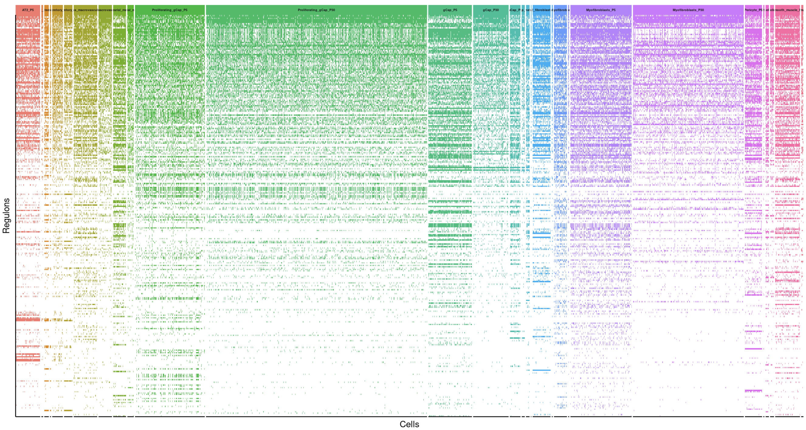

If you only want to check certain groups (ex: AT2_P5 and AT2_P30)

plot_tib3 <- plot_tib2[plot_tib2$celltype.timepoint == c("AT2_P5","AT2_P30"),]

bin_heatmap <- ggplot(data = plot_tib3, 
                      mapping = aes(x = cell_ID, y = regulon, fill = colcol)) +
  geom_tile() + 
  scale_fill_manual(values = myColors)  +
  theme(plot.background=element_blank(),
        axis.text.x=element_blank(),
        axis.text.y=element_blank(),
        axis.ticks.x=element_blank(),
        axis.ticks.y=element_blank()) + 
  theme(legend.position = "none") +
  facet_grid2(~factor(celltype.timepoint, 
                     levels = c("AT2_P5","AT2_P30",
                 "Ciliated_P5","Ciliated_P30",
                 "Secretory_P5","Secretory_P30",
                 "Venous_macrovascular_P5","Venous_macrovascular_P30",
                 "Venous_or_Artearial_macrovascular_P5","Venous_or_Artearial_macrovascular_P30",
                 "Proliferating_gCap_P5","Proliferating_gCap_P30",
                 "gCap_P5","gCap_P30",
                 "aCap_P5","aCap_P30",
                 "Lymphatic_P5","Lymphatic_P30",
                 "Wnt2_fibroblasts_P5","Wnt2_fibroblasts_P30",
                 "Prolif_Myofibroblasts_P5","Prolif_Myofibroblasts_P30",
                 "Myofibroblasts_P5","Myofibroblasts_P30",
                 "Pericyte_P5","Pericyte_P30",
                 "Mesothelium_P5","Mesothelium_P30",
                 "Smooth_muscle_P5","Smooth_muscle_P30")),
             scales = "free_x",
             space = "free_x",
             strip = strip)+
             #ncol = 30) + 
  theme(panel.spacing = unit(.1, "lines")) + 
  theme(axis.line = element_line(colour = "black"))+
  theme(strip.text.x = element_text(size = 4))+
  xlab("Cells")+
  ylab("Regulons")


bin_heatmap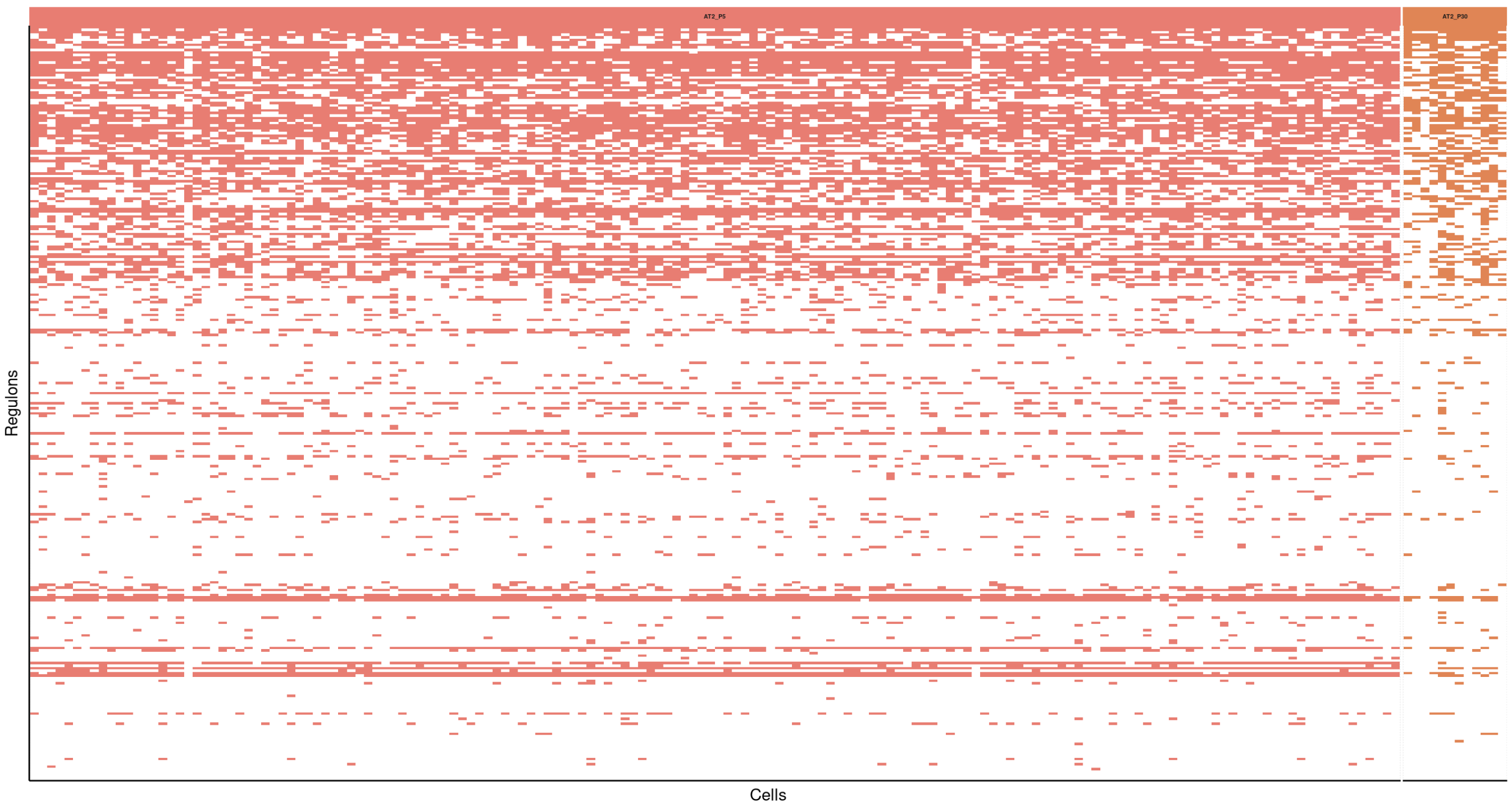

If, instead, I want to perform FindMarkers() to obtain DE regulons.

Gene order is determined by the avg_log2FC

# 只留下跟SCENIC_workflow_20230220一樣的 FindMarkers的 regulons
# gene order 也一樣是由avg_log2FC 的大小來排序


# 要先把 plot_tib 中 regulon的名字改成跟 SCENIC_workflow_20230220 一樣
plot_tib$regulon <- gsub("[(+)]", "", plot_tib$regulon)

# 只留下 FindMarker() 找到的 top20 genes
plot_tib3 <- dplyr::filter(plot_tib, regulon %in% top20$gene)


# gene order
plot_tib3$regulon <- factor(plot_tib3$regulon, levels = rev(gene_order))

# fill
plot_tib3 <- plot_tib3 %>% 
  mutate(colcol = ifelse(onoff == 1, as.character(celltype.timepoint), 0))


# plot
bin_heatmap <- ggplot(data = plot_tib3, 
                      mapping = aes(x = cell_ID, y = regulon, fill = colcol)) +
  geom_tile() + 
  scale_fill_manual(values = myColors)  +
  theme(plot.background=element_blank(),
        axis.text.x=element_blank(),
        axis.text.y=element_blank(),
        axis.ticks.x=element_blank(),
        axis.ticks.y=element_blank()) + 
  theme(legend.position = "none") +
  facet_grid2(~factor(celltype.timepoint, 
                     levels = c("AT2_P5","AT2_P30",
                 "Ciliated_P5","Ciliated_P30",
                 "Secretory_P5","Secretory_P30",
                 "Venous_macrovascular_P5","Venous_macrovascular_P30",
                 "Venous_or_Artearial_macrovascular_P5","Venous_or_Artearial_macrovascular_P30",
                 "Proliferating_gCap_P5","Proliferating_gCap_P30",
                 "gCap_P5","gCap_P30",
                 "aCap_P5","aCap_P30",
                 "Lymphatic_P5","Lymphatic_P30",
                 "Wnt2_fibroblasts_P5","Wnt2_fibroblasts_P30",
                 "Prolif_Myofibroblasts_P5","Prolif_Myofibroblasts_P30",
                 "Myofibroblasts_P5","Myofibroblasts_P30",
                 "Pericyte_P5","Pericyte_P30",
                 "Mesothelium_P5","Mesothelium_P30",
                 "Smooth_muscle_P5","Smooth_muscle_P30")),
             scales = "free_x",
             space = "free_x",
             strip = strip)+
             #ncol = 30) + 
  theme(panel.spacing = unit(.1, "lines")) + 
  theme(axis.line = element_line(colour = "black"))+
  theme(strip.text.x = element_text(size = 4))+
  xlab("Cells")+
  ylab("Regulons")


bin_heatmap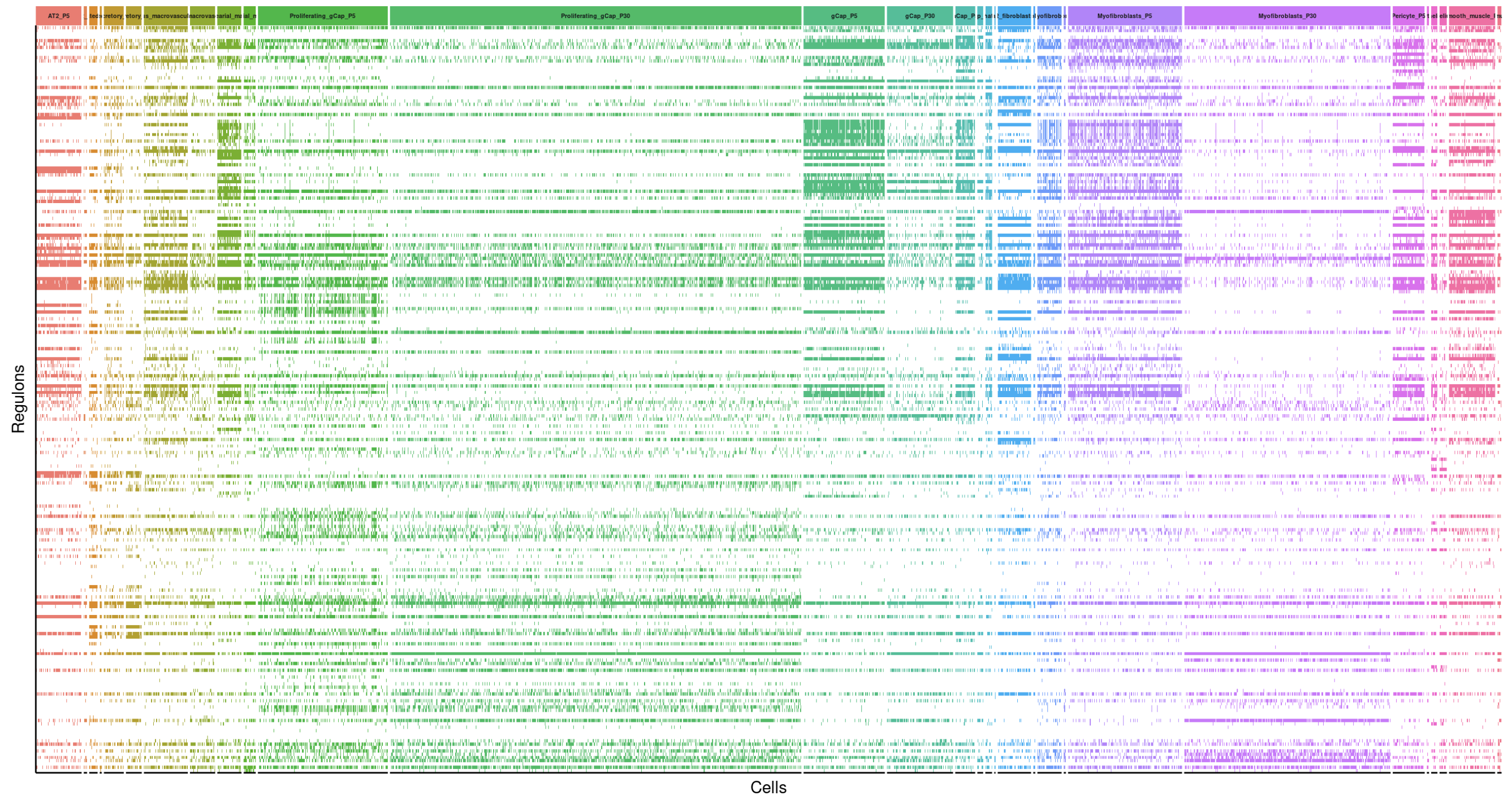

Gene order is determined by the number of cells expressing regulons

plot_tib$regulon <- gsub("[(+)]", "", plot_tib$regulon)
plot_tib3 <- dplyr::filter(plot_tib, regulon %in% top20$gene)


# gene order
reg_sum <- plot_tib3 %>%
  group_by(regulon) %>%
  summarise(total = sum(onoff == 1)) %>%
  arrange(desc(total))

plot_tib3$regulon <- factor(plot_tib3$regulon, levels = rev(reg_sum$regulon))

# fill
plot_tib3 <- plot_tib3 %>% 
  mutate(colcol = ifelse(onoff == 1, as.character(celltype.timepoint), 0))


# plot
bin_heatmap <- ggplot(data = plot_tib3, 
                      mapping = aes(x = cell_ID, y = regulon, fill = colcol)) +
  geom_tile() + 
  scale_fill_manual(values = myColors)  +
  theme(plot.background=element_blank(),
        axis.text.x=element_blank(),
        axis.text.y=element_blank(),
        axis.ticks.x=element_blank(),
        axis.ticks.y=element_blank()) + 
  theme(legend.position = "none") +
  facet_grid2(~factor(celltype.timepoint, 
                     levels = c("AT2_P5","AT2_P30",
                 "Ciliated_P5","Ciliated_P30",
                 "Secretory_P5","Secretory_P30",
                 "Venous_macrovascular_P5","Venous_macrovascular_P30",
                 "Venous_or_Artearial_macrovascular_P5","Venous_or_Artearial_macrovascular_P30",
                 "Proliferating_gCap_P5","Proliferating_gCap_P30",
                 "gCap_P5","gCap_P30",
                 "aCap_P5","aCap_P30",
                 "Lymphatic_P5","Lymphatic_P30",
                 "Wnt2_fibroblasts_P5","Wnt2_fibroblasts_P30",
                 "Prolif_Myofibroblasts_P5","Prolif_Myofibroblasts_P30",
                 "Myofibroblasts_P5","Myofibroblasts_P30",
                 "Pericyte_P5","Pericyte_P30",
                 "Mesothelium_P5","Mesothelium_P30",
                 "Smooth_muscle_P5","Smooth_muscle_P30")),
             scales = "free_x",
             space = "free_x",
             strip = strip)+
             #ncol = 30) + 
  theme(panel.spacing = unit(.1, "lines")) + 
  theme(axis.line = element_line(colour = "black"))+
  theme(strip.text.x = element_text(size = 4))+
  xlab("Cells")+
  ylab("Regulons")


bin_heatmap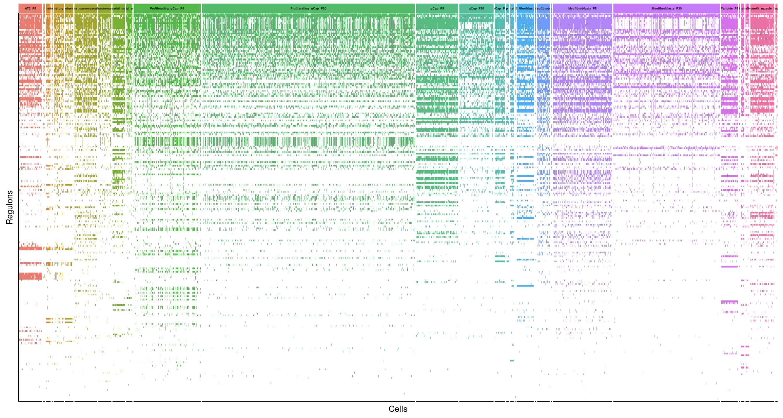

→ Feels like it is better to just visualize 2 treatments of certain subcelltype (e.g., AT2_P5 vs AT2_P30) →

4 versions of “AT2_P5 vs AT2_P30”

Do not filter out the regulons that express in cell number less than median(cell number).

#do not run:
# plot_tib2 <-plot_tib %>%
# group_by(regulon) %>%
# filter(sum(onoff) > median(FindMedian$total))

Versions

1. All genes from FindMarkers(); No hclust; Arrange the gene order with avg_log2FC.
2. Perform FindMarkers() on just AT2_P5 and AT2_P30, and collect all genes; No hclust; Arrange the gene order with avg_log2FC.
3. All genes from FindMarkers(); Perform hclust.
4. Perform FindMarkers() on just AT2_P5 and AT2_P30, and collect all genes; Perform hclust.

All genes from FindMarkers(); No hclust; Arrange the gene order with avg_log2FC.

plot_AT2 <- plot_tib[plot_tib$celltype.timepoint == c("AT2_P30", "AT2_P5"),]

# 只留下FindMarkers()找到的 regulons
plot_AT2$regulon <- gsub("[(+)]", "", plot_AT2$regulon)
plot_AT2 <- dplyr::filter(plot_AT2, regulon %in% top20$gene)


# gene order
gene_order <- top20 %>% arrange(desc(avg_log2FC))
gene_order <- unique(factor(gene_order$gene))
plot_AT2$regulon <- factor(plot_AT2$regulon, levels = rev(gene_order))


# fill
plot_AT2 <- plot_AT2 %>% 
  mutate(colcol = ifelse(onoff == 1, as.character(celltype.timepoint), 0))



# plot
bin_heatmap <- ggplot(data = plot_AT2, 
                      mapping = aes(x = cell_ID, y = regulon, fill = colcol)) +
  geom_tile() + 
  scale_fill_manual(values = myColors)  +
  theme(plot.background=element_blank(),
        axis.text.x=element_blank(),
        axis.text.y=element_blank(),
        axis.ticks.x=element_blank(),
        axis.ticks.y=element_blank()) + 
  theme(legend.position = "none") +
  facet_grid2(~factor(celltype.timepoint, 
                     levels = c("AT2_P5","AT2_P30",
                 "Ciliated_P5","Ciliated_P30",
                 "Secretory_P5","Secretory_P30",
                 "Venous_macrovascular_P5","Venous_macrovascular_P30",
                 "Venous_or_Artearial_macrovascular_P5","Venous_or_Artearial_macrovascular_P30",
                 "Proliferating_gCap_P5","Proliferating_gCap_P30",
                 "gCap_P5","gCap_P30",
                 "aCap_P5","aCap_P30",
                 "Lymphatic_P5","Lymphatic_P30",
                 "Wnt2_fibroblasts_P5","Wnt2_fibroblasts_P30",
                 "Prolif_Myofibroblasts_P5","Prolif_Myofibroblasts_P30",
                 "Myofibroblasts_P5","Myofibroblasts_P30",
                 "Pericyte_P5","Pericyte_P30",
                 "Mesothelium_P5","Mesothelium_P30",
                 "Smooth_muscle_P5","Smooth_muscle_P30")),
             scales = "free_x",
             space = "free_x",
             strip = strip)+
             #ncol = 30) + 
  theme(panel.spacing = unit(.1, "lines")) + 
  theme(axis.line = element_line(colour = "black"))+
  theme(strip.text.x = element_text(size = 8))+
  xlab("Cells")+
  ylab("Regulons")


bin_heatmap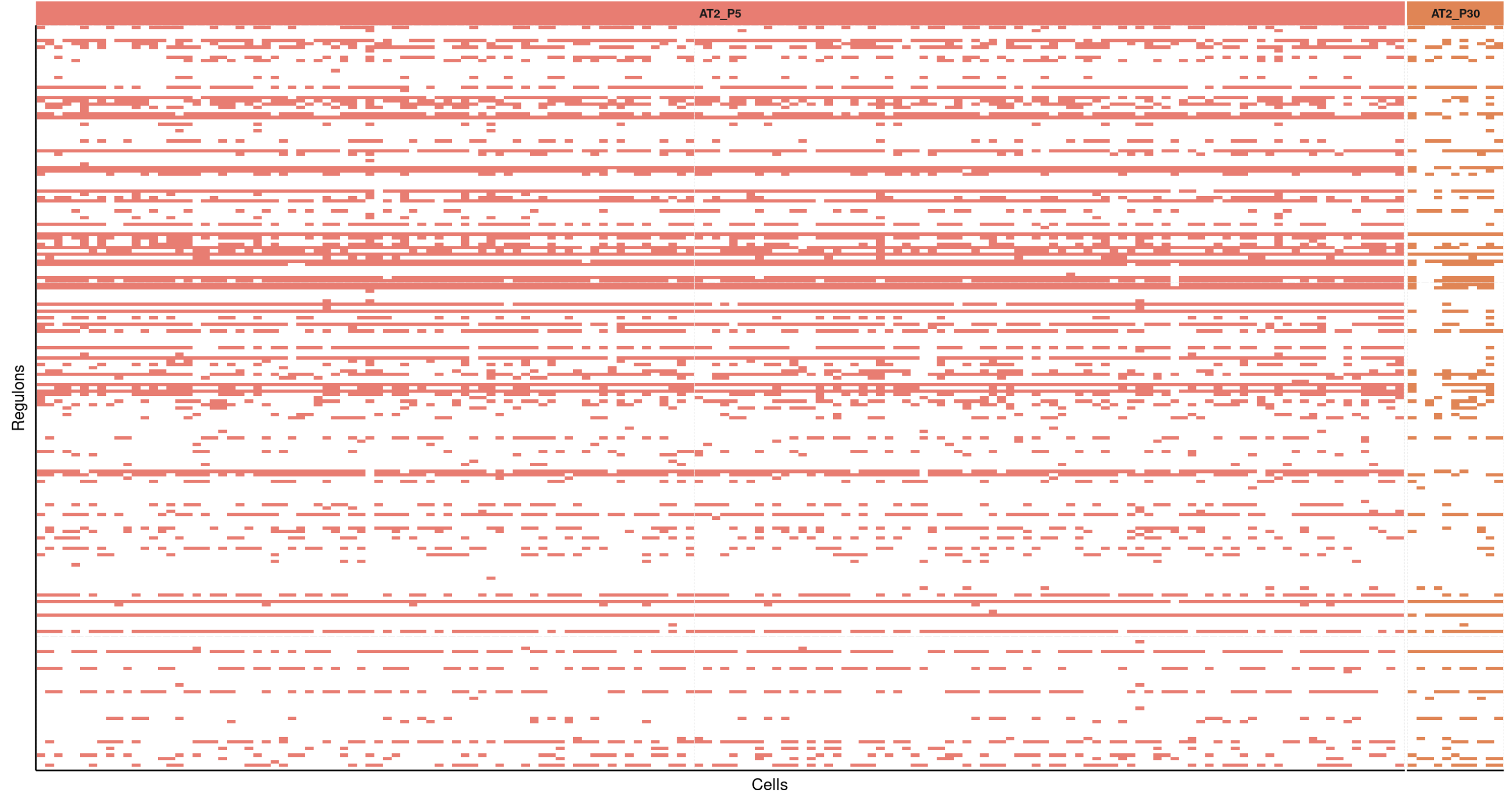

Perform FindMarkers() on just AT2_P5 and AT2_P30, and collect all genes; No hclust; Arrange the gene order with avg_log2FC.

plot_AT2 <- plot_tib[plot_tib$celltype.timepoint == c("AT2_P30", "AT2_P5"),]

# 只留下FindMarkers()找到的 regulons
plot_AT2$regulon <- gsub("[(+)]", "", plot_AT2$regulon)
plot_AT2 <- dplyr::filter(plot_AT2, regulon %in% AT2_gene$gene)


# AT2 gene order
AT2_gene <- top20[top20$subcelltype %in% c("AT2_P5","AT2_P30"),]
AT2_gene_order <- AT2_gene %>% arrange(desc(avg_log2FC))
AT2_gene_order <- unique(factor(AT2_gene_order$gene))
plot_AT2$regulon <- factor(plot_AT2$regulon, levels = rev(AT2_gene_order))



# fill
plot_AT2 <- plot_AT2 %>% 
  mutate(colcol = ifelse(onoff == 1, as.character(celltype.timepoint), 0))



# plot
bin_heatmap <- ggplot(data = plot_AT2, 
                      mapping = aes(x = cell_ID, y = regulon, fill = colcol)) +
  geom_tile() + 
  scale_fill_manual(values = myColors)  +
  theme(plot.background=element_blank(),
        axis.text.x=element_blank(),
        axis.text.y=element_blank(),
        axis.ticks.x=element_blank(),
        axis.ticks.y=element_blank()) + 
  theme(legend.position = "none") +
  facet_grid2(~factor(celltype.timepoint, 
                     levels = c("AT2_P5","AT2_P30",
                 "Ciliated_P5","Ciliated_P30",
                 "Secretory_P5","Secretory_P30",
                 "Venous_macrovascular_P5","Venous_macrovascular_P30",
                 "Venous_or_Artearial_macrovascular_P5","Venous_or_Artearial_macrovascular_P30",
                 "Proliferating_gCap_P5","Proliferating_gCap_P30",
                 "gCap_P5","gCap_P30",
                 "aCap_P5","aCap_P30",
                 "Lymphatic_P5","Lymphatic_P30",
                 "Wnt2_fibroblasts_P5","Wnt2_fibroblasts_P30",
                 "Prolif_Myofibroblasts_P5","Prolif_Myofibroblasts_P30",
                 "Myofibroblasts_P5","Myofibroblasts_P30",
                 "Pericyte_P5","Pericyte_P30",
                 "Mesothelium_P5","Mesothelium_P30",
                 "Smooth_muscle_P5","Smooth_muscle_P30")),
             scales = "free_x",
             space = "free_x",
             strip = strip)+
             #ncol = 30) + 
  theme(panel.spacing = unit(.1, "lines")) + 
  theme(axis.line = element_line(colour = "black"))+
  theme(strip.text.x = element_text(size = 8))+
  xlab("Cells")+
  ylab("Regulons")


bin_heatmap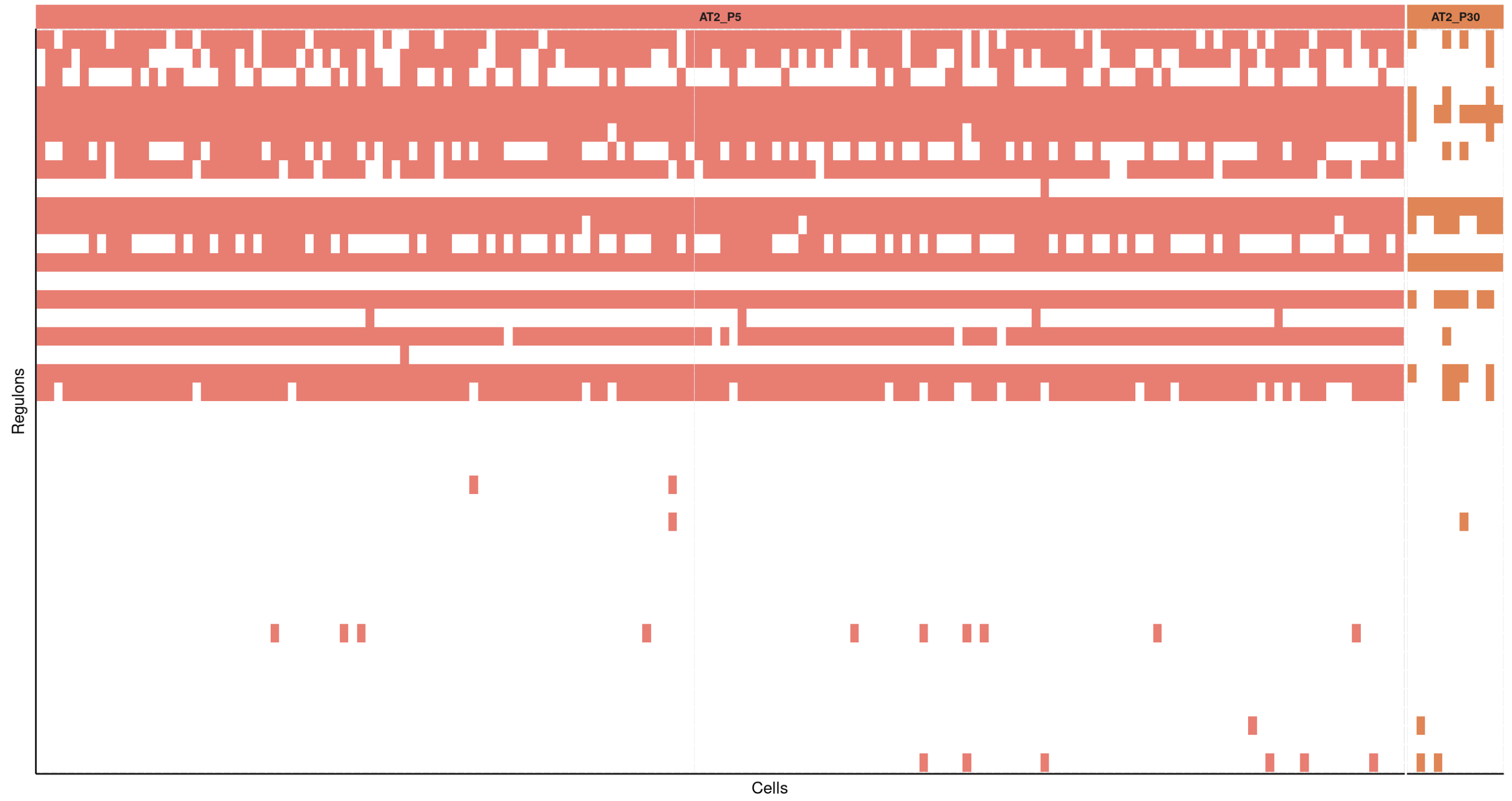

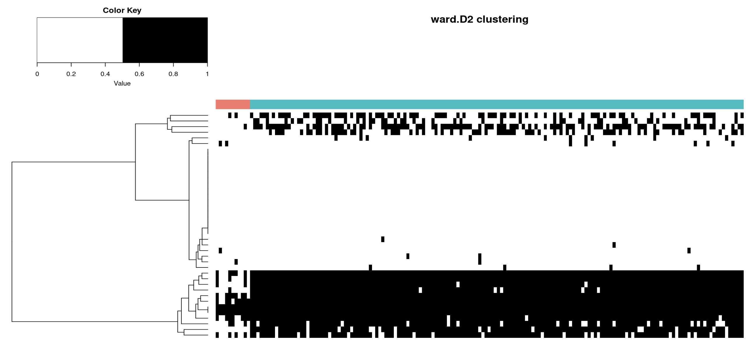
All genes from FindMarkers(); Perform hclust.

plot_AT2 <- plot_tib[plot_tib$celltype.timepoint == c("AT2_P30", "AT2_P5"),]


# 只留下FindMarkers()找到的 regulons
plot_AT2$regulon <- gsub("[(+)]", "", plot_AT2$regulon)
plot_AT2 <- dplyr::filter(plot_AT2, regulon %in% top20$gene)


plot_AT2_wide <- reshape2::dcast(plot_AT2, 
                       regulon ~ cell_ID, 
                       value.var = "onoff")

rownames(plot_AT2_wide) <- plot_AT2_wide$regulon
plot_AT2_wide$regulon <- NULL




# clustering
hr <- hclust(amap::Dist(plot_AT2_wide, method = "euclidean"), method = "ward.D2")
mycl <- cutree(hr,  h = 50/100*max(hr$height))
mycolhc <- rainbow(length(unique(mycl)), start=1, end=0.5)
mycolhc <- mycolhc[as.vector(mycl)]
myheatcol <- c("#FFFFFF","#000000")


# heatmap



gplots::heatmap.2(as.matrix(plot_AT2_wide),
          Rowv=as.dendrogram(hr),
          Colv = F,
          col=myheatcol,
          scale="none",
          density.info="none",
          trace="none",
         # RowSideColors=mycolhc,
          labRow = F,
          labCol = F,
          ColSideColors=rep(scales::hue_pal()(2), 
                            c(length(grep("P30_", colnames(plot_AT2_wide))),
                              length(grep("P5_", colnames(plot_AT2_wide))))),
          main="ward.D2 clustering")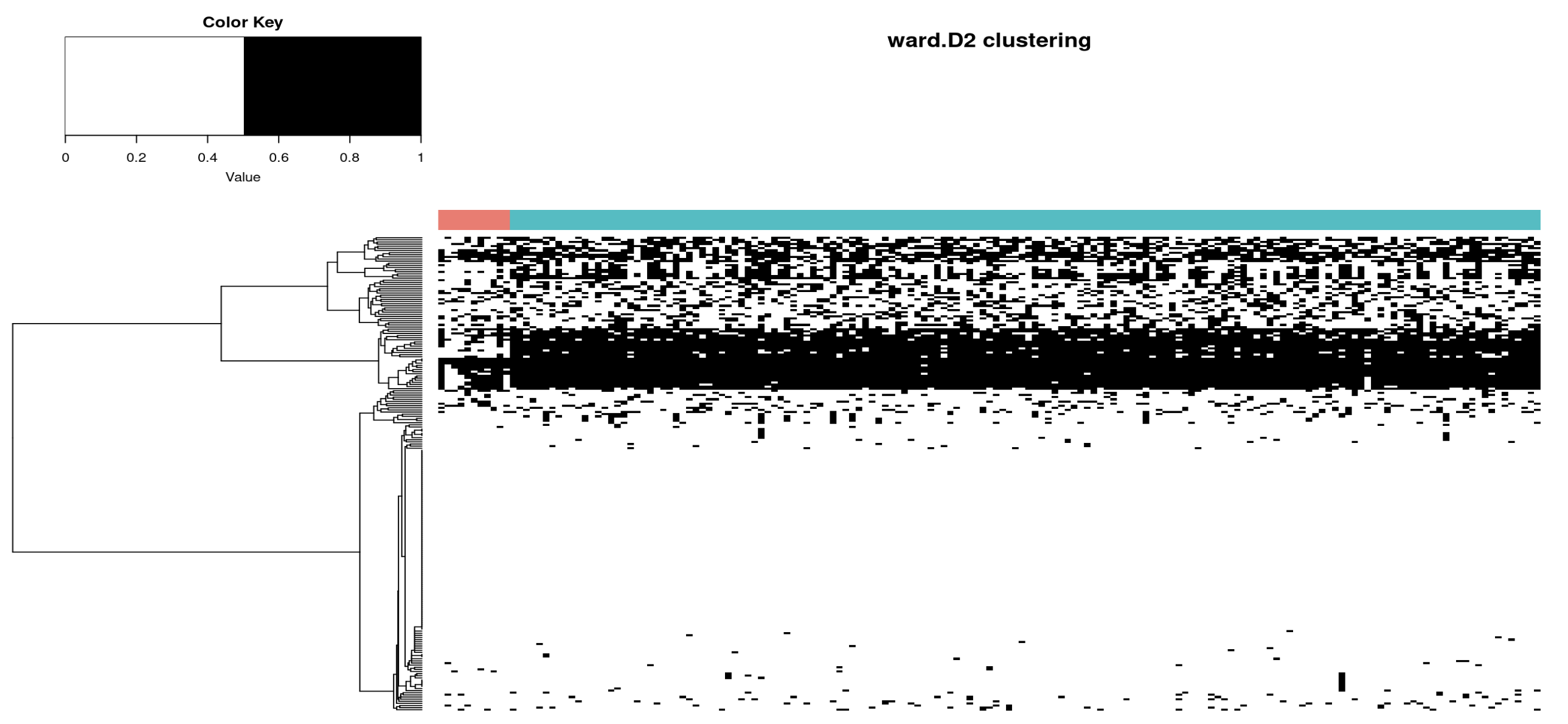

Perform FindMarkers() on just AT2_P5 and AT2_P30, and collect all genes; Perform hclust.

plot_AT2 <- plot_tib[plot_tib$celltype.timepoint == c("AT2_P30", "AT2_P5"),]

AT2_gene <- top20[top20$subcelltype %in% c("AT2_P5","AT2_P30"),]

# 只留下FindMarkers()找到的 regulons
plot_AT2$regulon <- gsub("[(+)]", "", plot_AT2$regulon)
plot_AT2 <- dplyr::filter(plot_AT2, regulon %in% AT2_gene$gene)


plot_AT2_wide <- reshape2::dcast(plot_AT2, 
                       regulon ~ cell_ID, 
                       value.var = "onoff")

rownames(plot_AT2_wide) <- plot_AT2_wide$regulon
plot_AT2_wide$regulon <- NULL




# clustering
hr <- hclust(amap::Dist(plot_AT2_wide, method = "euclidean"), method = "ward.D2")
mycl <- cutree(hr,  h = 50/100*max(hr$height))
mycolhc <- rainbow(length(unique(mycl)), start=1, end=0.5)
mycolhc <- mycolhc[as.vector(mycl)]
myheatcol <- c("#FFFFFF","#000000")


# heatmap



gplots::heatmap.2(as.matrix(plot_AT2_wide),
          Rowv=as.dendrogram(hr),
          Colv = F,
          col=myheatcol,
          scale="none",
          density.info="none",
          trace="none",
         # RowSideColors=mycolhc,
          labRow = F,
          labCol = F,
          ColSideColors=rep(scales::hue_pal()(2), 
                            c(length(grep("P30_", colnames(plot_AT2_wide))),
                              length(grep("P5_", colnames(plot_AT2_wide))))),
          main="ward.D2 clustering")