0. How does DESeq2 normalize data?
DESeq2 size-factor normalization does not adjust for gene length
Size-factor calculation
Calculate SIZE FACTOR
- Dividing each gene’s read count by the geometric mean of read counts for that gene across all samples.
read_count_A / sqrt(read_count_A * read_count_B) = ratio_read_count_A
Ratio_A = ReadCount_A / sqrt(ReadCount_A × ReadCount_B) - For each sample, the median of these ratios (after excluding genes with zero counts in any sample) is used as the sample’s size factor.
Norm_A = ReadCount_A / median(Ratios)Normalization With the size factors at hand, DESeq2 normalizes the read counts for each gene in each sample by dividing the raw counts by the sample’s size factor. This step adjusts for differences in sequencing depth and RNA composition between samples, allowing for an apples-to-apples comparison.
1. Why do we need to know about dispersion?
To accurately model sequencing counts, we need to generate accurate estimates of within-group variation (variation between replicates of the same sample group) for each gene. With only three to six biological replicates, gene-wise estimates of variation can be unreliable, and genes with similar means may have substantially different dispersion estimates.
Sharing information across genes
DESeq2 shares information across genes to generate more accurate estimates of variation based on the mean expression level of the gene using a method called ‘shrinkage’. The dispersion trend uses the relationship between mean expression and dispersion across genes. The initial gene-wise dispersion estimates are obtained by maximum likelihood estimation.
2. What is dispersion? How to interpret plotDispEsts?
Dispersion describes variability beyond the Poisson component of the negative-binomial count model. It is related to variation among replicates, but it is not identical to variance or standard deviation. The fitted trend often decreases with mean expression: lowly expressed genes tend to show more relative variation and stochasticity in their measurements. Lower dispersion indicates that replicates are very similar, whereas higher dispersion suggests more variability among replicates.
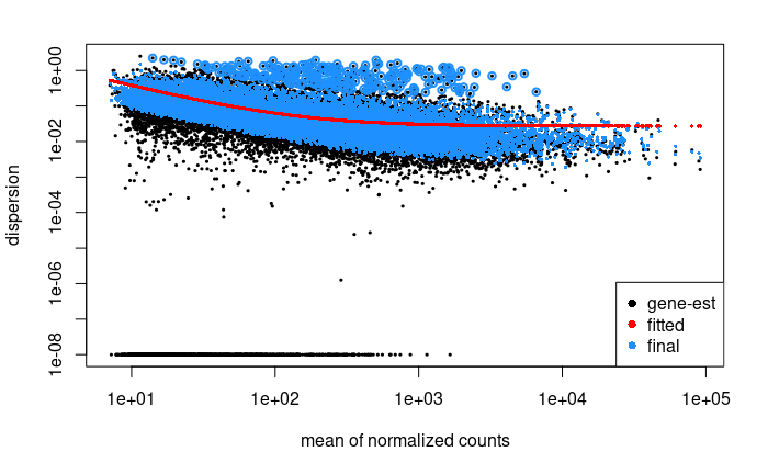
- The y-axis shows dispersion estimates.
- The red line is the fitted mean–dispersion trend obtained from genes across the expression range.
- Gene-wise estimates are shrunk towards the trend (blue points). High-dispersion outliers may retain their gene-wise estimates rather than being pulled towards the trend (circled points).
- More stable dispersion estimates support better-calibrated downstream differential-expression testing.
3. Why variance stabilizing transformation (VST)?
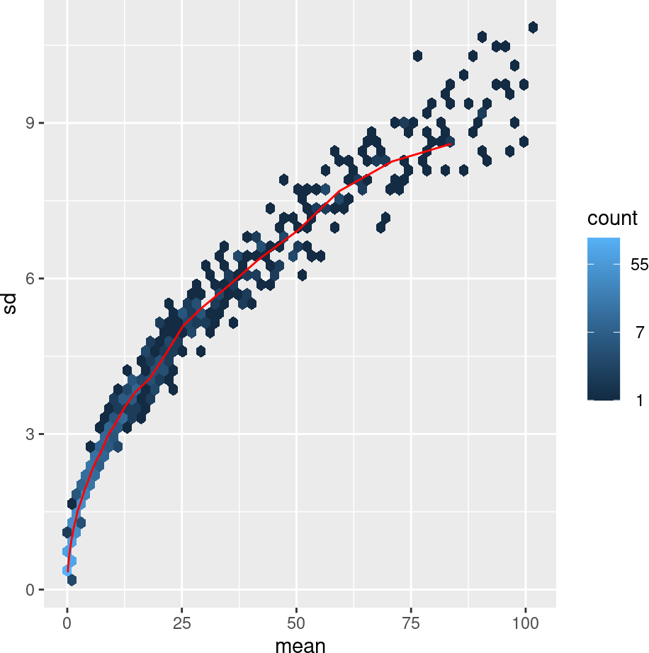
For PCA, it is useful to reduce the dependence of the variance on the mean expression level. Raw RNA-seq counts usually show increasing variance as the mean increases. The figure below illustrates the wider spread at high mean counts. Without a suitable transformation, sample distances can be dominated by genes with the largest means, because they also have the largest absolute differences between samples.
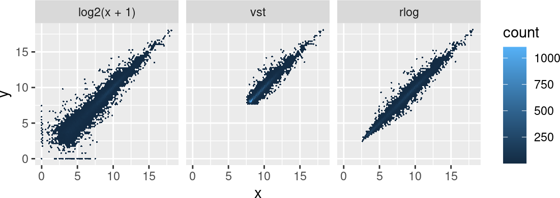
A log(x + 1) transformation is one option, but its pseudocount can strongly affect low-count genes. Those genes can contribute disproportionately to sample distances and PCA despite a low signal-to-noise ratio.
Variance stabilizing transformation
DESeq2’s VST uses the fitted dispersion relationship to reduce the dependence of variance on the mean; it is intended for visualization and exploratory analyses, rather than as the input to the differential-expression test. The aim is a transformed matrix with approximately comparable variance across the range of mean expression values, especially at low means.
4. What is lfcShrink?
in short, it looks at the largest fold changes that are not due to low counts and uses these to inform a prior distribution. So the large fold changes from genes with lots of statistical information are not shrunk, while the imprecise fold changes are shrunk. This allows you to compare all estimated LFC across experiments, for example, which is not really feasible without the use of a prior.