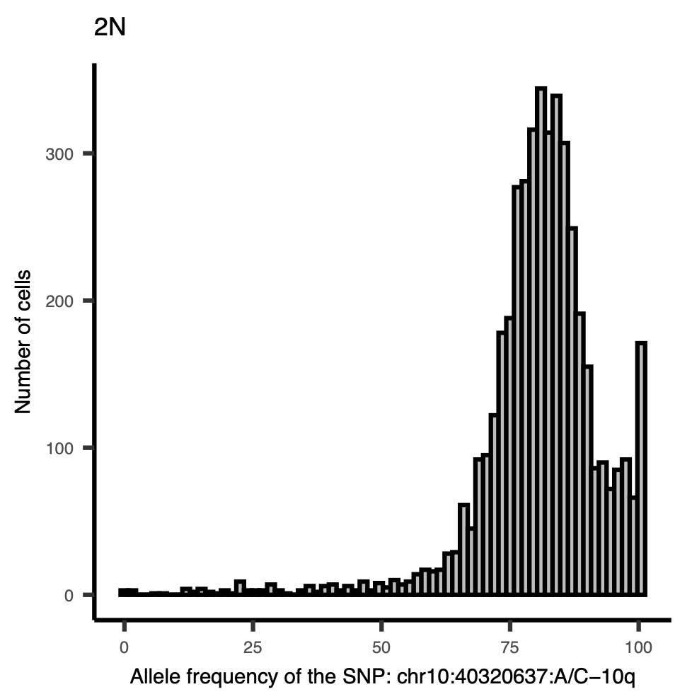
The input dataframe contains 4,478 cells × 62 SNPs.
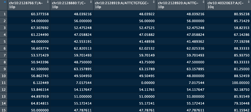
Distribution plots
Plot a distribution for every column, with the number of cells on the y-axis.

For each column, count values at both ends of the distribution: values equal to 0 or 100, values ≤1 or ≥99, values ≤2 or ≥98, and so on.
Define a tail-ratio function for each SNP
For lower = 0 and upper = 100, count values ≤0 or ≥100 in each column and divide by the number of values to obtain a ratio.
column_ValueOutOfRangeRatio <- function(matrix,
                                  lower_criteria = 0,
                                  higher_criteria = 100
                                  ){

  result = data.frame(row.names = colnames(matrix))
  result[,1] = 0
  colnames(result) = paste0("Ratio_",lower_criteria,"_",higher_criteria)

     # for loop for each SNPs
     for (i in 1:ncol(matrix)){

     count = sum(matrix[,i] <= lower_criteria |  matrix[,i] >= higher_criteria)
     ratio = round((count/nrow(matrix))*100, digits = 2)

     # Find the row_index of the current SNPs in the data frame
     row_index <- match(colnames(matrix)[i], rownames(result))

     result[row_index, colnames(result)] <- ratio

     }

  return(result)

}
Evaluate several lower and upper cutoffs
AF_62_mtx_2N <- AF_62_mtx_2N[,-c(1:2)]


# for loop for different range (i+j has to be 100)
SNP_AlleleFreqOutOfRangeRatios <- data.frame(row.names = colnames(AF_62_mtx_2N))
for (i in 0:10) {
  j = 100 - i

  new_df <- column_ValueOutOfRangeRatio(AF_62_mtx_2N,
                                        lower_criteria = i,
                                        higher_criteria = j)
  SNP_AlleleFreqOutOfRangeRatios = cbind(SNP_AlleleFreqOutOfRangeRatios, new_df)

  }
Compare tail ratios with a line chart
Code
SNP_AlleleFreqOutOfRangeRatios$SNPs <- rownames(SNP_AlleleFreqOutOfRangeRatios)

# conver to long format
SNP_AlleleFreqOutOfRangeRatios_long <- tidyr::pivot_longer(data = SNP_AlleleFreqOutOfRangeRatios,
                                                           cols = -c(SNPs),
                                                           names_to = "range",
                                                           values_to = "ratio")
# make sure the order of x axis (range character)
SNP_AlleleFreqOutOfRangeRatios_long$range <- factor(SNP_AlleleFreqOutOfRangeRatios_long$range,
                                                       levels = unique(SNP_AlleleFreqOutOfRangeRatios_long$range))


####################################################################################
# Visualization
pdf(file = "PDF/QC/2N_SNP_AlleleFreqOutOfRangeRatios.pdf", width = 10, height = 6)

# chr3, 6, 7, 8
ggplot(SNP_AlleleFreqOutOfRangeRatios_long[grep("chr3|chr6|chr7|chr8",
                                                SNP_AlleleFreqOutOfRangeRatios_long$SNPs,
                                                ignore.case = TRUE),],
       aes(x = range,
           y = ratio,
           group = SNPs)) +
  geom_line(aes(color = SNPs))+
  geom_point(aes(color = SNPs))+
  theme_classic() +
  theme(text = element_text(size=15),
        axis.text.x = element_text(angle = 45, vjust = 1, hjust=1))+
  ggtitle("Ratios of allele frequency that are out of range: chr3,chr6,chr7,chr8")

# chr10
ggplot(SNP_AlleleFreqOutOfRangeRatios_long[grep("chr10",
                                                SNP_AlleleFreqOutOfRangeRatios_long$SNPs,
                                                ignore.case = TRUE),],
       aes(x = range,
           y = ratio,
           group = SNPs)) +
  geom_line(aes(color = SNPs))+
  geom_point(aes(color = SNPs))+
  theme_classic() +
  theme(text = element_text(size=15),
        axis.text.x = element_text(angle = 45, vjust = 1, hjust=1))+
  ggtitle("Ratios of allele frequency that are out of range: chr10")


# chr11, 12, 13
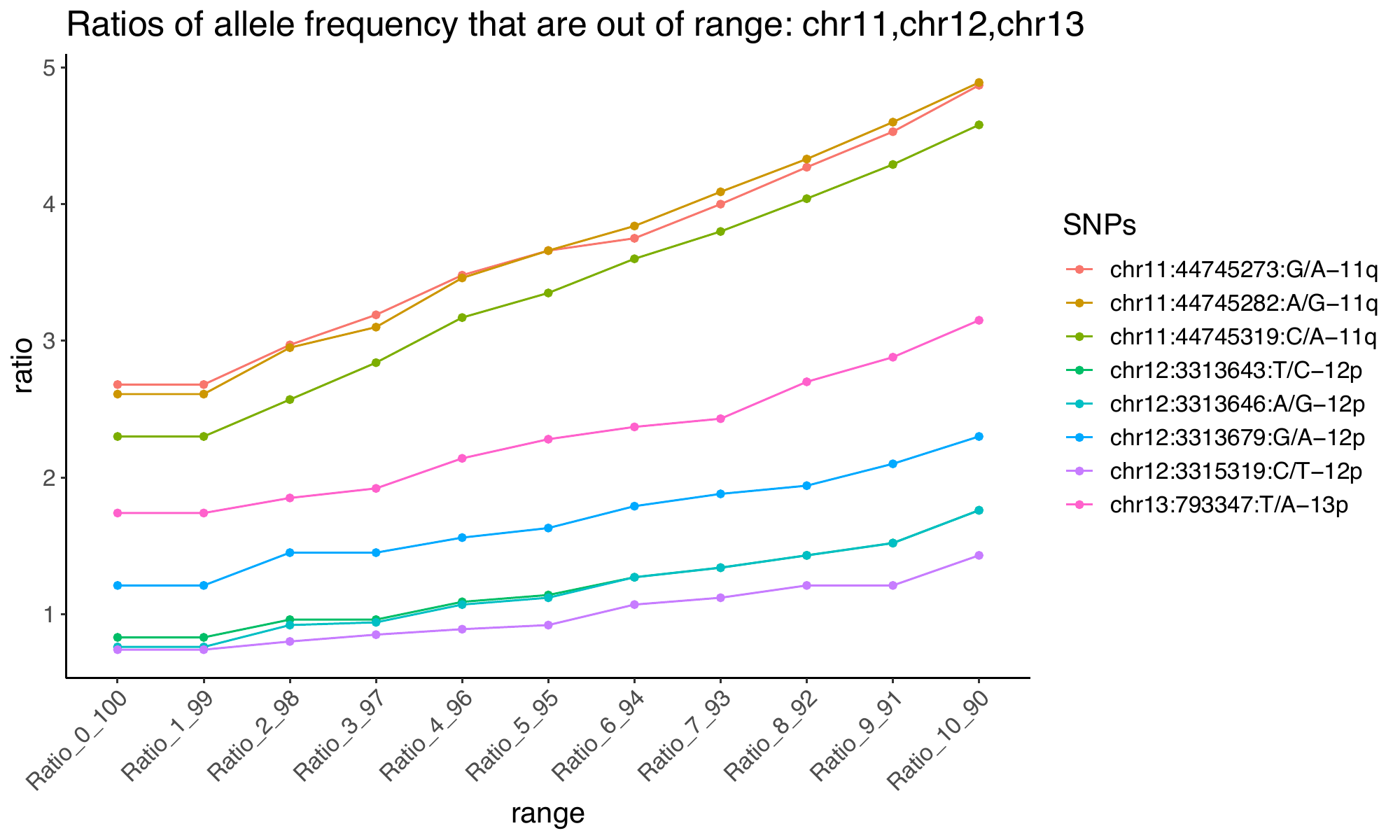
ggplot(SNP_AlleleFreqOutOfRangeRatios_long[grep("chr11|chr12|chr13",
                                                SNP_AlleleFreqOutOfRangeRatios_long$SNPs,
                                                ignore.case = TRUE),],
       aes(x = range,
           y = ratio,
           group = SNPs)) +
  geom_line(aes(color = SNPs))+
  geom_point(aes(color = SNPs))+
  theme_classic() +
  theme(text = element_text(size=15),
        axis.text.x = element_text(angle = 45, vjust = 1, hjust=1))+
  ggtitle("Ratios of allele frequency that are out of range: chr11,chr12,chr13")


# chr14
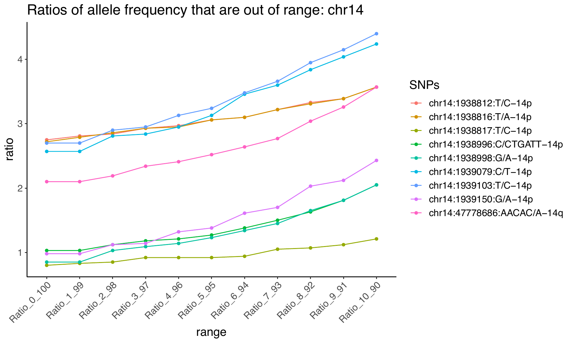
ggplot(SNP_AlleleFreqOutOfRangeRatios_long[grep("chr14", SNP_AlleleFreqOutOfRangeRatios_long$SNPs, ignore.case = TRUE),],
       aes(x = range,
           y = ratio,
           group = SNPs)) +
  geom_line(aes(color = SNPs))+
  geom_point(aes(color = SNPs))+
  theme_classic() +
  theme(text = element_text(size=15),
        axis.text.x = element_text(angle = 45, vjust = 1, hjust=1))+
  ggtitle("Ratios of allele frequency that are out of range: chr14")


# chr15
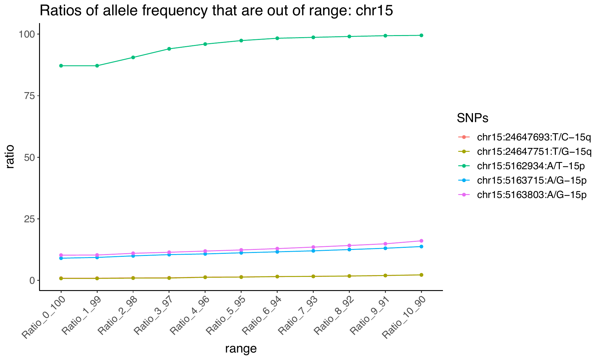
ggplot(SNP_AlleleFreqOutOfRangeRatios_long[grep("chr15",
                                                SNP_AlleleFreqOutOfRangeRatios_long$SNPs,
                                                ignore.case = TRUE),],
       aes(x = range,
           y = ratio,
           group = SNPs)) +
  geom_line(aes(color = SNPs))+
  geom_point(aes(color = SNPs))+
  theme_classic() +
  theme(text = element_text(size=15),
        axis.text.x = element_text(angle = 45, vjust = 1, hjust=1))+
  ggtitle("Ratios of allele frequency that are out of range: chr15")


# chr16, 17
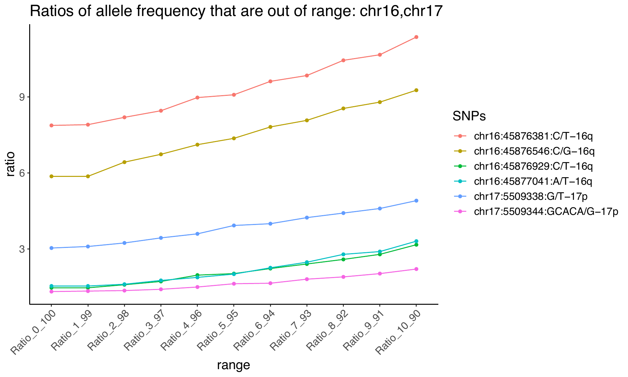
ggplot(SNP_AlleleFreqOutOfRangeRatios_long[grep("chr16|chr17",
                                                SNP_AlleleFreqOutOfRangeRatios_long$SNPs,
                                                ignore.case = TRUE),],
       aes(x = range,
           y = ratio,
           group = SNPs)) +
  geom_line(aes(color = SNPs))+
  geom_point(aes(color = SNPs))+
  theme_classic() +
  theme(text = element_text(size=15),
        axis.text.x = element_text(angle = 45, vjust = 1, hjust=1))+
  ggtitle("Ratios of allele frequency that are out of range: chr16,chr17")


# chr18, 19
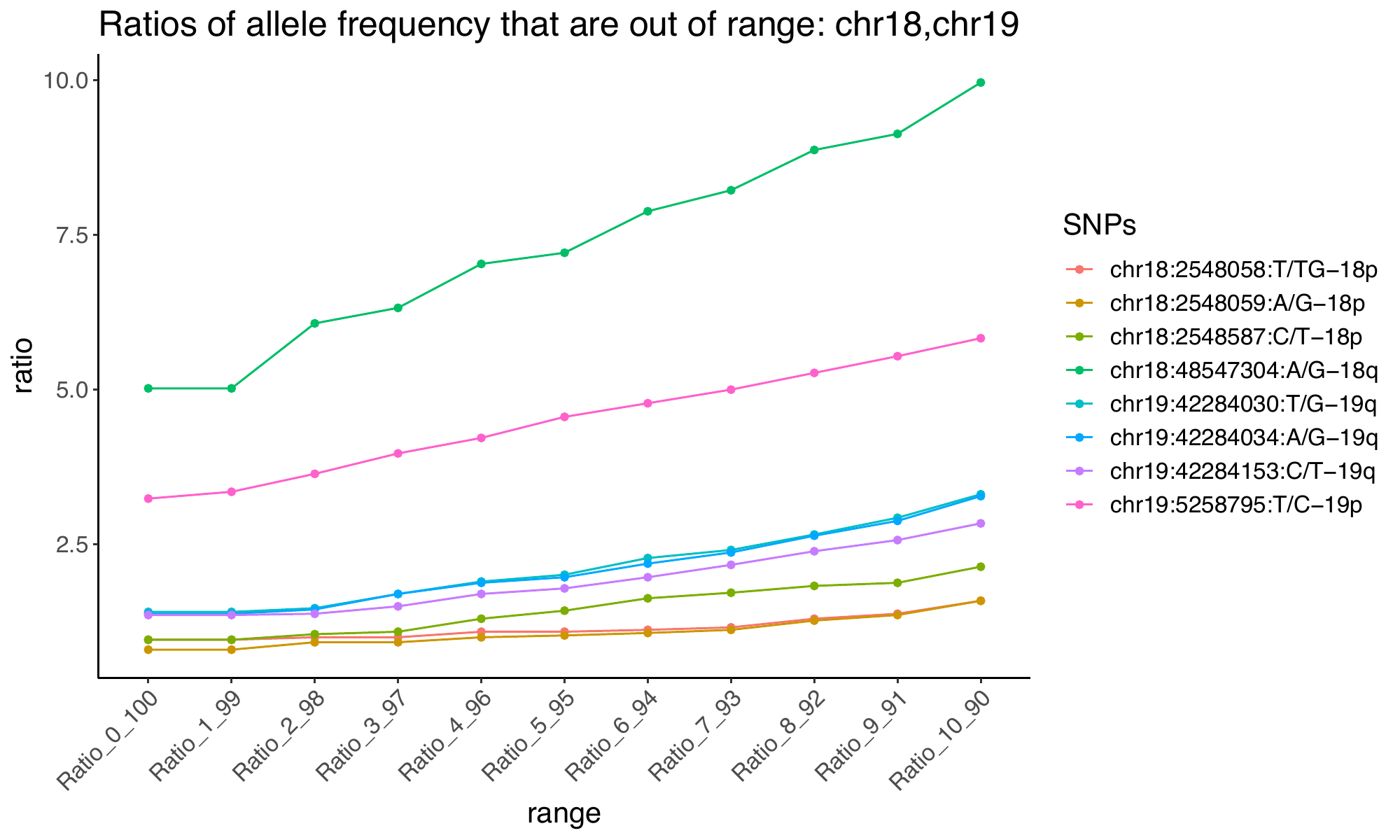
ggplot(SNP_AlleleFreqOutOfRangeRatios_long[grep("chr18|chr19",
                                                SNP_AlleleFreqOutOfRangeRatios_long$SNPs,
                                                ignore.case = TRUE),],
       aes(x = range,
           y = ratio,
           group = SNPs)) +
  geom_line(aes(color = SNPs))+
  geom_point(aes(color = SNPs))+
  theme_classic() +
  theme(text = element_text(size=15),
        axis.text.x = element_text(angle = 45, vjust = 1, hjust=1))+
  ggtitle("Ratios of allele frequency that are out of range: chr18,chr19")

# chr21
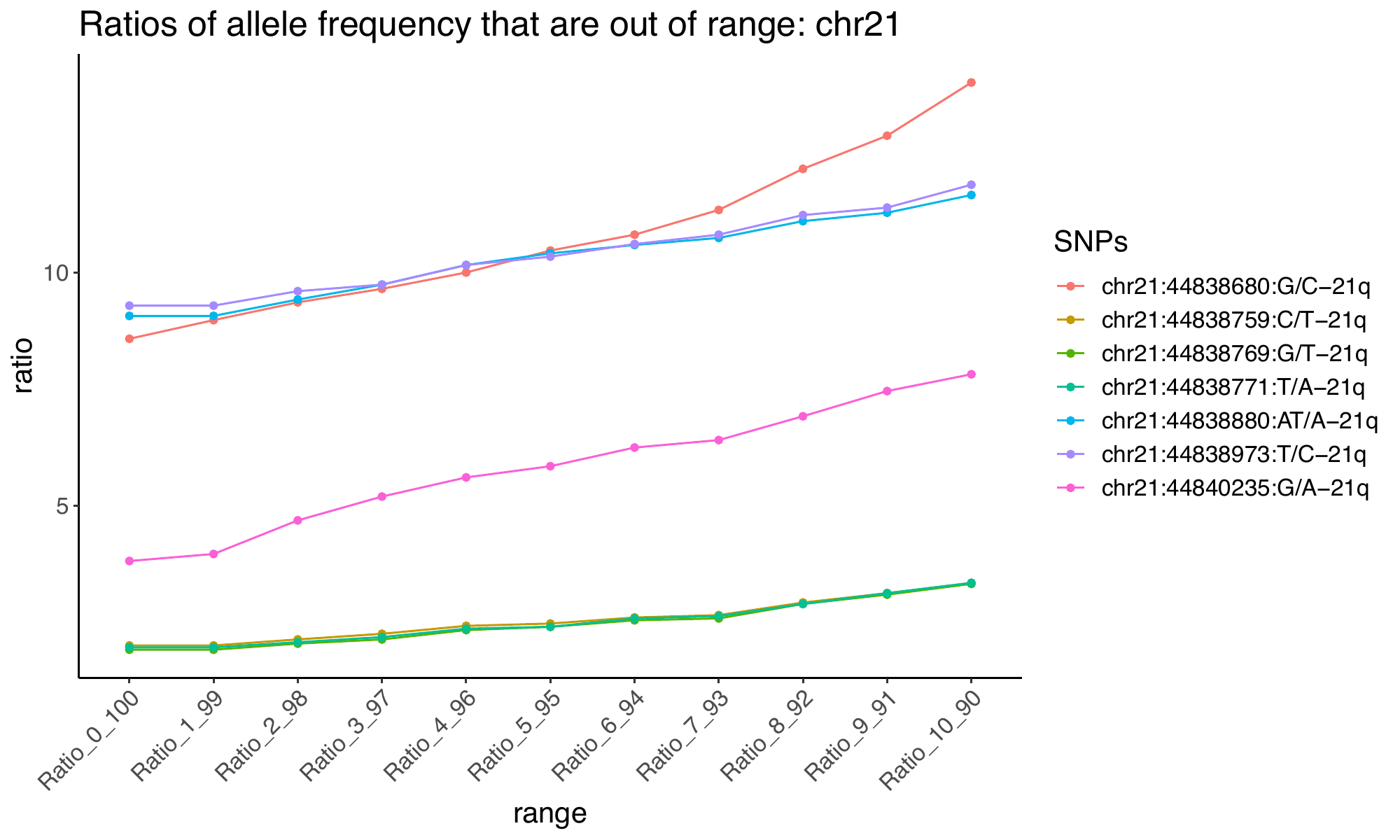
ggplot(SNP_AlleleFreqOutOfRangeRatios_long[grep("chr21",
                                                SNP_AlleleFreqOutOfRangeRatios_long$SNPs,
                                                ignore.case = TRUE),],
       aes(x = range,
           y = ratio,
           group = SNPs)) +
  geom_line(aes(color = SNPs))+
  geom_point(aes(color = SNPs))+
  theme_classic() +
  theme(text = element_text(size=15),
        axis.text.x = element_text(angle = 45, vjust = 1, hjust=1))+
  ggtitle("Ratios of allele frequency that are out of range: chr21")


# chr22, 25
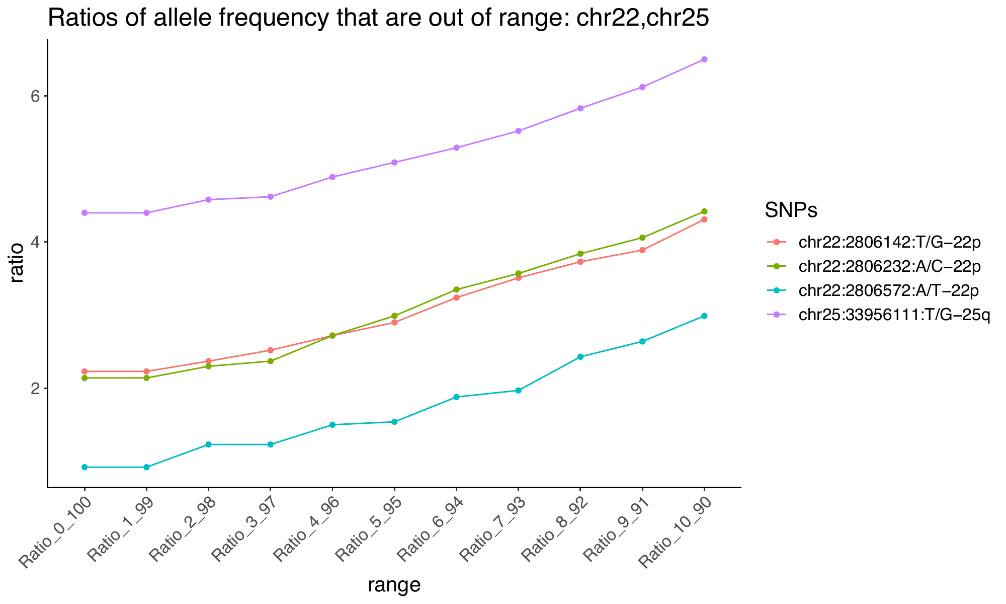
ggplot(SNP_AlleleFreqOutOfRangeRatios_long[grep("chr22|chr25",
                                                SNP_AlleleFreqOutOfRangeRatios_long$SNPs,
                                                ignore.case = TRUE),],
       aes(x = range,
           y = ratio,
           group = SNPs)) +
  geom_line(aes(color = SNPs))+
  geom_point(aes(color = SNPs))+
  theme_classic() +
  theme(text = element_text(size=15),
        axis.text.x = element_text(angle = 45, vjust = 1, hjust=1))+
  ggtitle("Ratios of allele frequency that are out of range: chr22,chr25")

dev.off()
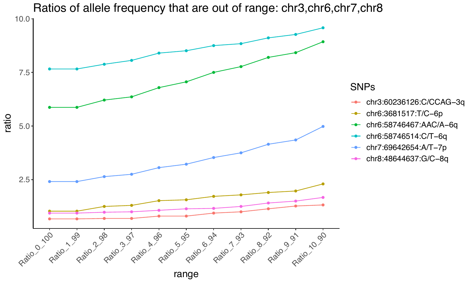
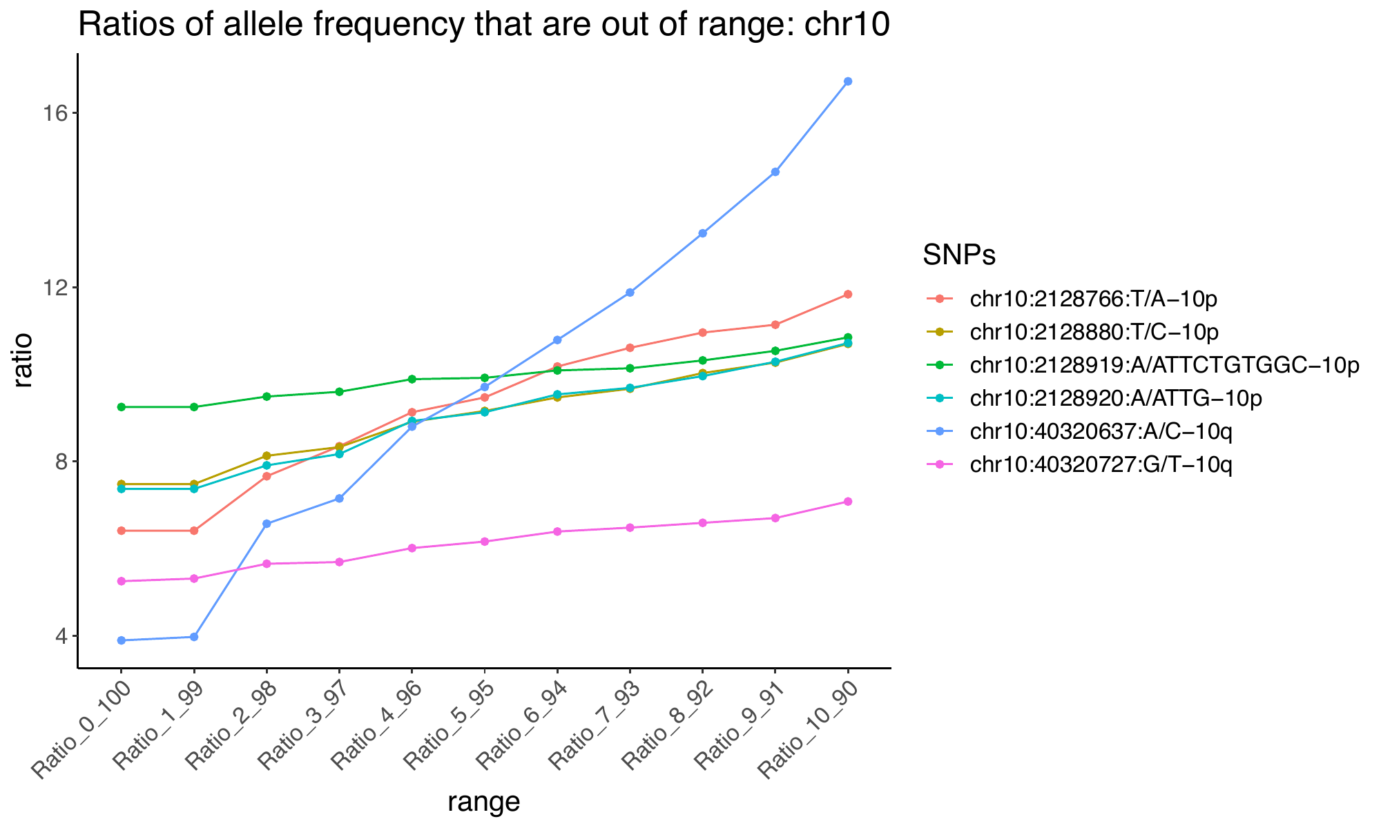
Each line represents one column (one SNP).
The y-axis is the proportion outside the chosen range; the x-axis identifies the range. For example, Ratio_10_90 is the proportion of values ≤10 or ≥90.
2N_SNP_AlleleFreqOutOfRangeRatios.pdf
Summary
The curves compare the tail proportions across SNPs and show how rapidly those proportions increase as the central interval narrows. The SNP chr10:40320637:A/C−10q has a notably different pattern.
Its histogram below also shows an asymmetric distribution.